Optimizing a simple ray-tracer written in Go, part 1

04 July 2020 // Erik Lupander

In this 2-part blog we’ll take a look at how I used the go profiling and built-in benchmarking tools to optimize a naive ray-tracer written in Go.

Click here for Part 2.

Contents

1. Introduction
2. Why Go?
3. Multi-threading
4. Using pprof to identify bottlenecks
5. Reducing allocations & Caching
6. Conclusion of part 1

(Note: Most of this blog post is based on using Go 1.13)

Source code

The full source code for my little ray-tracer can be found here: https://github.com/eriklupander/rt

1. Introduction

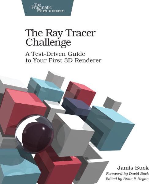
Sometime late 2019 I stumbled upon a book - “The Ray Tracer Challenge”:

What is ray-tracing? Let’s quote wikipedia:

In computer graphics, ray tracing is a rendering technique for generating 
an image by tracing the path of light as pixels in an image plane and 
simulating the effects of its encounters with virtual objects. 

Source: https://en.wikipedia.org/wiki/Ray_tracing(graphics)_

Professional ray-tracing can produce quite photo-realistic results: Source: https://en.wikipedia.org/wiki/Ray_tracing(graphics)#/media/File:Glasses_800edit.png

While ray-tracing has approximately 0% relation to my daily work, I’ve been interested in computer graphics ever since the mid-late 80’s when I wrote my first GW BASIC graphics code and played any computer game on the family 286 I could lay my hands upon.

Ray tracing has always been something of my personal holy grail of computer graphics. I’ve toyed around with rasterization in the past, doing some OpenGL and shader stuff just for fun, but given the mathematical nature of ray tracing, I’ve never really even tried to wrap my head around it. You can never guess what happened next when I discovered the book above…

1.1 The Ray Tracer Challenge

A few words on the book that launched me onto the path of writing my very own ray-tracer. The book in question takes a fully language-agnostic approach to building your very own ray-tracer from scratch. The book does a really good job expaining the physics and mathematics involved without drowning the reader in mathematical formulas or equations. While a number of key algorithms are explained both using plain text and imperative psuedo-code, the heart of the book is its test-driven approach where concepts are first explain in text, and then defined as cucumber-like Given - When - Then test cases. Example:

        test: normal on a child object
		Given g1 ← group()
		And set_transform(g1, rotation_y(π/2))
		And g2 ← group()
		And set_transform(g2, scaling(1, 2, 3))
		And add_child(g1, g2)
		And s ← sphere()
		And set_transform(s, translation(5, 0, 0))
		And add_child(g2, s)
		When n ← normal_at(s, point(1.7321, 1.1547, -5.5774))
		Then n = vector(0.2857, 0.4286, -0.8571)

Everything from intersection math, rotations, linear algebra, shading to lighting calculations has these test cases to keep you as the reader of the book on the correct path. Which is enormously important, best stated in the book in regard to getting the basics wrong early on:

"... it will cause you a never-ending series of headaches"

- Jamis Buck, The Ray Tracer Challenge

Indeed - if you’d get some fundamental piece of the core math or intersection algorithms wrong, later use of those functions (such as checking intersections of a ray) will be off and very difficult to troubleshoot.

So, the book takes you step by step from building your core math library, rendering your first pixels and grasping the core concepts - to actually rendering various shapes including lighting, reflections, refraction, shadows etc. By the end of the book, your renderer is capable of creating images such as the one below: 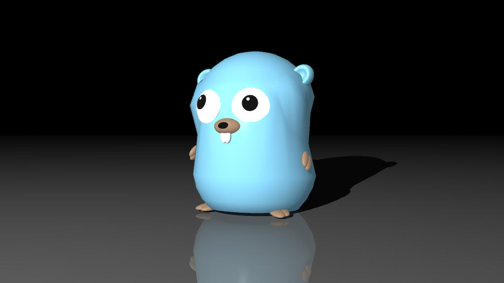Gopher model by Takuya Ueda

That said - the purpose of this blog post is not teaching you how to create a ray-tracer - buy the book instead. This blog post is about Golang and my journey after finishing the book making my renderer perform better. As it turned out, my performance optimizations cut the time for a single render by several orders of magnitude!

1.2 The “reference” image

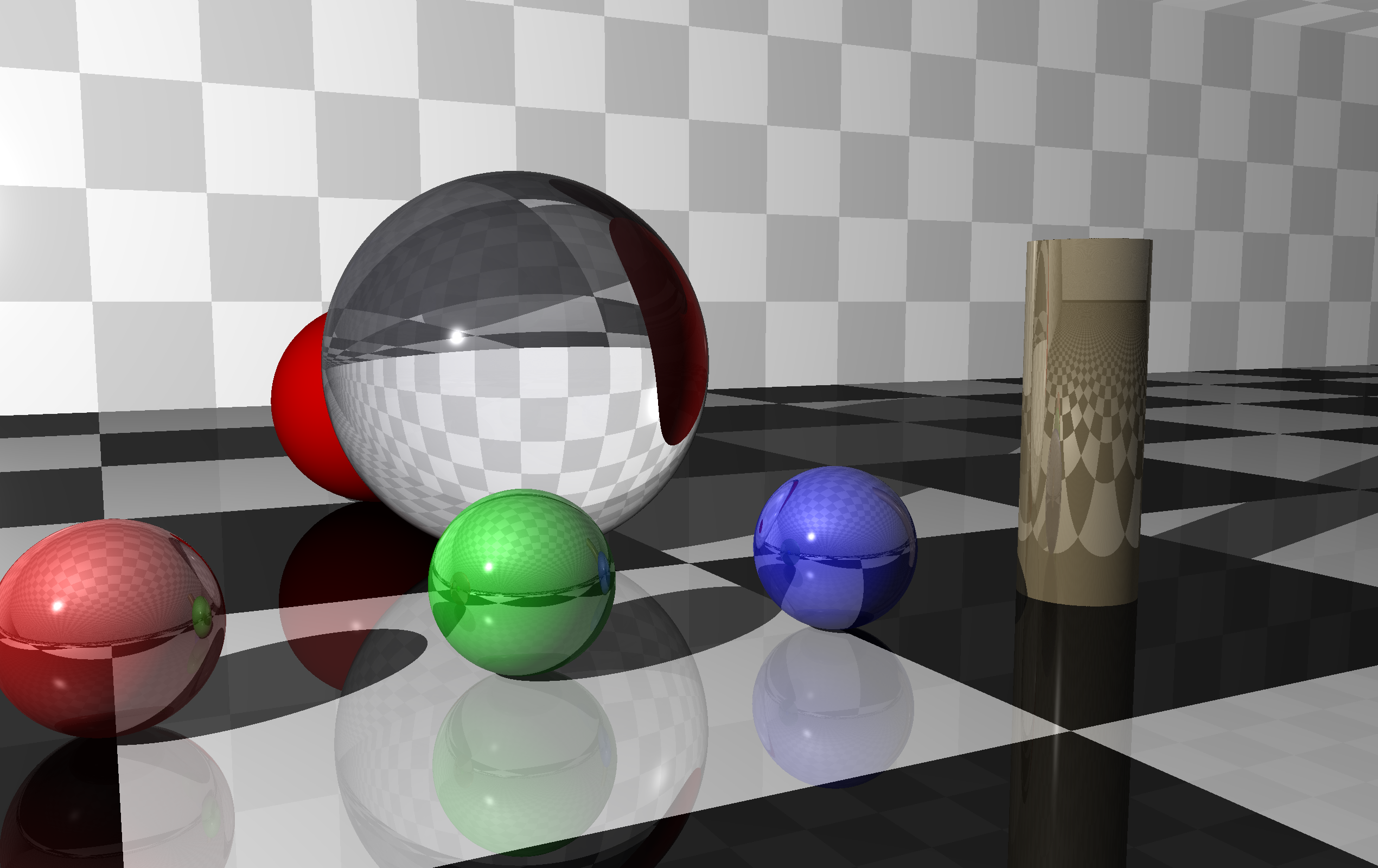While not very impressive given 2020 graphical standards, this “reference image” of mine showcases a number of different object primitives, shadows, reflections, refraction, lighting, patterns and transparency. This is a high-res render, while the resolution used for all performance comparisons were 640x480.

2. Why Go?

Why not? Ok - after doing Java for 15+ years, I’ve been working full-time with Go projects for the last year or so. And I simply love the simplicity of the language, the fast and efficient tooling and how the language manages to make our team able to efficiently write stable, performant and correct services without having the language or its abstractions getting in our way very often.

I’ll also admit - if I had wanted to write the most performant ray-tracer from the very beginning, I probably should have done this in C, C++ or Rust. However, given that my challenge was learning how to do simple ray-tracing, I’d rather not have to deal with (re)learning a programming language I’m not comfortable with. This point is actually rather significant, as it turned out I’ve probably spent more time on my ray-tracer after finishing the book doing the performance optimizations this blog post is about than I spent with the book. Nevertheless, it’s quite probable I’d run into many or most of the issues in whatever language I’d picked.

The cucumber-like tests from the book was implemented as standard Go unit tests. My implementation using Go 1.13 used no 3rd party libraries at the time I completed the book.

2.1 Other optimizations

This blog post is about improving the Go-related code of the renderer. However, I must clarify that a huge part of creating a performant ray-tracer is actually about making it “do less work” through optimization of the actual logic of the renderer. Ray-tracing is mainly about casting rays and checking if they intersect something. If you can decrease the number of rays to cast without sacrificing image quality, that is probably the greatest improvement you can do.

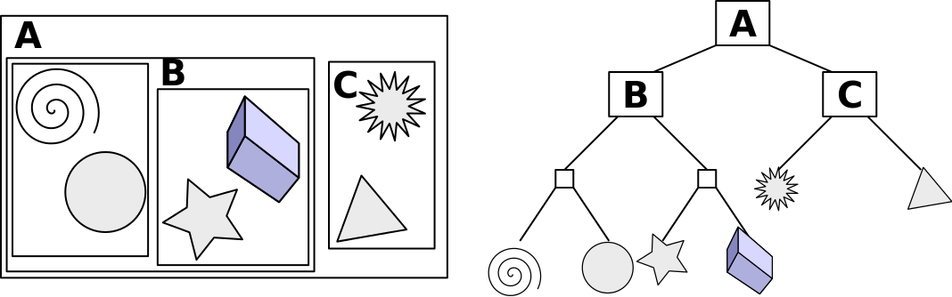
An example of such an improvement is using something called Bounding Boxes, where a complex object is encapsulated inside a “cheap” primitive, which can speed up rendering of complex meshes by several orders of magnitude:

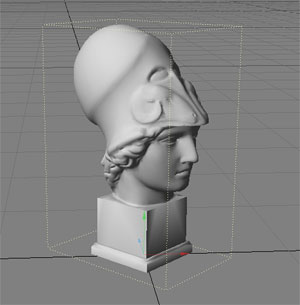
(Source Wikimedia: https://commons.wikimedia.org/wiki/File:BoundingBox.jpg)

A complex mesh such as the head in the image above may consist of hundreds of thousands of triangles. Without optimizations, a naive ray tracer would need to do an intersection test for every single triangle for for every ray cast in the scene, including shadow and reflection rays. That would make rendering of complex scenes quite infeasible on commodity hardware, where a single render could probably stretch into days or weeks to finish. Instead, by putting the complex head mesh inside a virtual “box”, a simple ray-box intersection test for each ray cast will tell us whether we need to test all the triangles of the head or not. I.e. - if the ray doesn’t intersect the box, it won’t intersect any of the thousands of triangles either so we can skip them.

Further, we can subdivide the head into many smaller boxes in a tree-like structure we can traverse and only do intersection tests for the triangles bounded by the leaf “box”. This is known as bounding volume hierarchies.

Source: Wikimedia: https://commons.wikimedia.org/wiki/File:Example_of_bounding_volume_hierarchy.svg)

As said above - these optimizations are tremendously important for complex scenes with many and/or complex objects. While I’ve implemented Bounding Boxes and BVHs in my renderer based on one of the online bonus chapters of the book, for the simple “reference image” used for benchmarking in this blog post, the BVH is ineffectual since the reference scene does not contain any grouped primitives.

3. Multi-threading

Once I was done with the book, I could render simple scenes such as the “reference image” on my MacBook Pro 2014 (4 core / 8 thread) in 640x480 resolution in about 3 minutes and 15 seconds. This made further experimentations with multi-sampling, textures or soft shadows a very slow process, leading to me embarking upon my journey of optimizations.

At a glance, ray-tracing is more or less about casting a ray through each would-be pixel through the image plane, and then applying the exact same algorithms for determining the output color of that given pixel. In theory, this sounds like an embarrassingly parallell problem.

Therefore, my first optimization was to move from a purely single-threaded rendering process to something that would utilize all available CPU threads.

3.1 Distributing the work

So, this is where the Go fun starts. I decided to apply the simple worker pool pattern that I’ve touched on before on this blog.

In terms of Go code, the renderer treats each horizontal line of pixels as a unit of work that one of the workers can consume from a channel. The number of workers is set to GOMAXPROCS, matching the number of virtual CPU cores, 4/8 in my case.

// Use a wait-group to wait until all lines have been rendered, adding HEIGHT (such as 480) to the waitGroup.
wg := sync.WaitGroup{}
wg.Add(canvas.H)

// Create the render contexts, one per worker. A render context is a struct with the requisite methods and scene info to render pixels.
renderContexts := make([]Context, config.Cfg.Threads)
for i := 0; i < config.Cfg.Threads; i++ {
    renderContexts[i] = NewContext(i, worlds[i], c, canvas, jobs, &wg)
}

// start workers
for i := 0; i < config.Cfg.Threads; i++ {
    go renderContexts[i].workerFuncPerLine()
}

// start passing work to the workers over the "jobs" channel, one line at a time
for row := 0; row < c.Height; row++ {
    jobs <- &job{row: row, col: 0}
}

wg.Wait()

The actual rendering code (e.g. workerFuncPerLine()) just picks one “job” at a time from the channel and passes it to our renderPixelPinhole method:

func (rc *Context) workerFuncPerLine() {
	for job := range rc.jobs {
		for i := 0; i < rc.camera.Width; i++ {
			job.col = i
			rc.renderPixelPinhole(job)
		}
		rc.wg.Done()
	}
}

3.2 Unit of work - congestion issues?

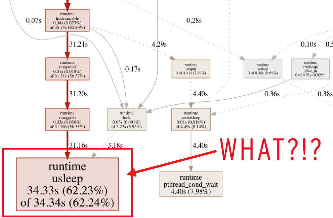
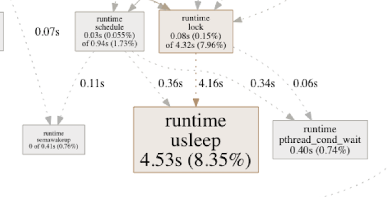
Why use one line as the unit of work? Well, actually, I started passing one pixel at a time. However, if you’re rendering a 1920x1080 image, that’s approx 2 million “jobs” to pass over that channel. I noticed in a CPU profile run that a large portion of time was being spent in this runtime.usleep method:

(Partial profile, pass one pixel per job)

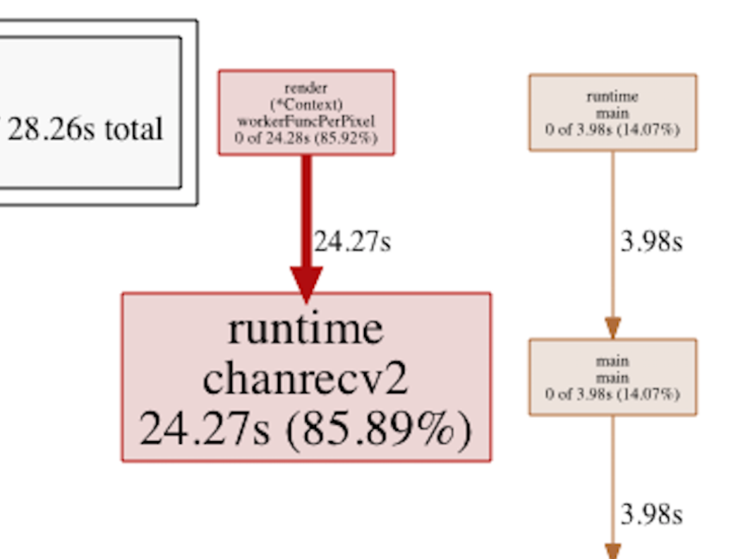
I couldn’t quite make sense of this, other than the profiling tools seemed to think a ridiculous amount of time was being spent waiting for something. A block profile shed some additional light on the issue:

(Block profile, pass one pixel per job)

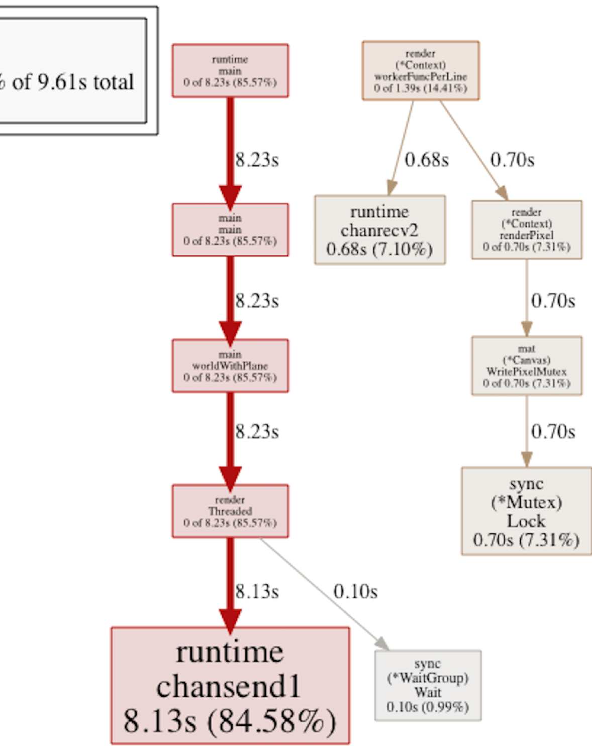
Seems the workerFuncPerLine() method spent a whole lot of time being blocked. By performing the tiny change of passing a line at a time instead of a single pixel as the unit of work, things started looking much better:

(Block profile, pass one line per job)

In this particular example, the block in chanrcv2 went from 34.3 seconds down to 0.6, while the chansend1 actually increased from 4 to 8 seconds, clearly indicating the we improved things a lot while simultaneously moving the bottleneck to the sender side. The CPU profile also looked much better now:

(Profile, pass one line per job)

Overall - one should notice that this change didn’t cut the total render time in half, it yielded an overall improvement of perhaps 5-7% - but it’s a good example on how an issue could be identified using the Golang profiling tools not directly related to mathematics or ray-tracing algorithms, rather a problem with the internal app architecture and how “jobs” were distributed to the “workers”.

3.3 Sharing memory

As I quite quickly noticed, moving the codebase from strict single-threaded operation to using a worker pool introduced a whole new slew of problems to solve. State and shared object structures was definitely one of the more challenging ones.

What does the code that renders a single pixel need to do its job? Well, it needs to access all geometry and light sources in the scene, as well as knowing where the “camera” is. All that stuff was implemented as plain Go structs, including quite a bit of state that at times was being mutated by the renderer in order to avoid allocating memory for intermediate calculations.

This was actually a bit harder nut to crack than I initially thought. Since I didn’t fancy rewriting everything from scratch, and using mutexes everywhere would both be error-prone and probably wouldn’t scale all that well - I decided to let each “render thread” get a full copy of the entire scene to work with. As long as the scene doesn’t contain a lot of really complex 3D models, in this day of 16GB laptops keeping N number of “copies” of some structs in-memory isn’t a big issue.

The final declaration of a “Render Context” is implemented as a Go struct and looks like this:

type Context struct {
	world  mat.World           // All objects and lights in the scene
	camera mat.Camera          // The camera representation
	canvas *mat.Canvas         // The output canvas where the final color of each pixel is written
	jobs   chan *job           // Channel that the "jobs" are passed over
	wg     *sync.WaitGroup     // Synchronizing so we know when all workers are done
	depth  int                 // Keeping track of recursion depth
}

The renderer instantiates GOMAXPROCS number of these “render contexts” that can autonomously render any pixel in the scene. Perhaps not the most elegant of solutions, but it provided safety and did definitely solve some of the rather strange render errors and other problems I did get before moving away from “shared memory”.

Whenever a pixel had been completed, it was directly written to the *mat.Canvas through a mutex-protected method. This mutex did not become any kind of bottleneck.

3.4 Running multi-threaded

So, how did going from 1 to 8 “workers” affect performance? While I didn’t expect my renders to become 8 times faster, I was kind of expecting maybe a 5-7x speedup.

I got about 2.5x.

The reference image was down to about 1m30s from 3m15s. This was a huge disappointment! But on the flip side, it really got me intrigued about what was holding the CPU back. I’ll revisit this in the final section of the second blog post of this mini-series.

4. pprof and reducing allocations

What do you do when your code doesn’t perform like you expect? You profile it! So, I added the requisite boilerplate to enable profiling:

import (
	...
	_ "net/http/pprof"
	...
)

func main() {
	// ... other code ...
	runtime.SetBlockProfileRate(1)
	runtime.SetMutexProfileFraction(1)
	// Enable PPROF web server
	go func() {
		log.Println(http.ListenAndServe("localhost:6060", nil))
	}()

I guess the finer details of pprof is better explained elsewhere, so let’s jump directly to what the CPU profile showed after enabling multi-threading:

These profile PNGs are awesome for seeing not only where the most time is being spent (hint - bigger is NOT better) but also the call hierarchies. Seems about 25% of the CPU time was being spent on runtime.mallocgc, which in plain english means “stuff the Garbage Collector is doing”. While my naive ray-tracer definitely wasn’t written with memory re-use in mind, this did seem a bit excessive.

Luckily, the profiling tools also provides heap profiling capable of both tracking the amount of memory being allocated down to LoC level, as well as showing the number of allocations occurring in any given function or LoC.

Time for a big image:

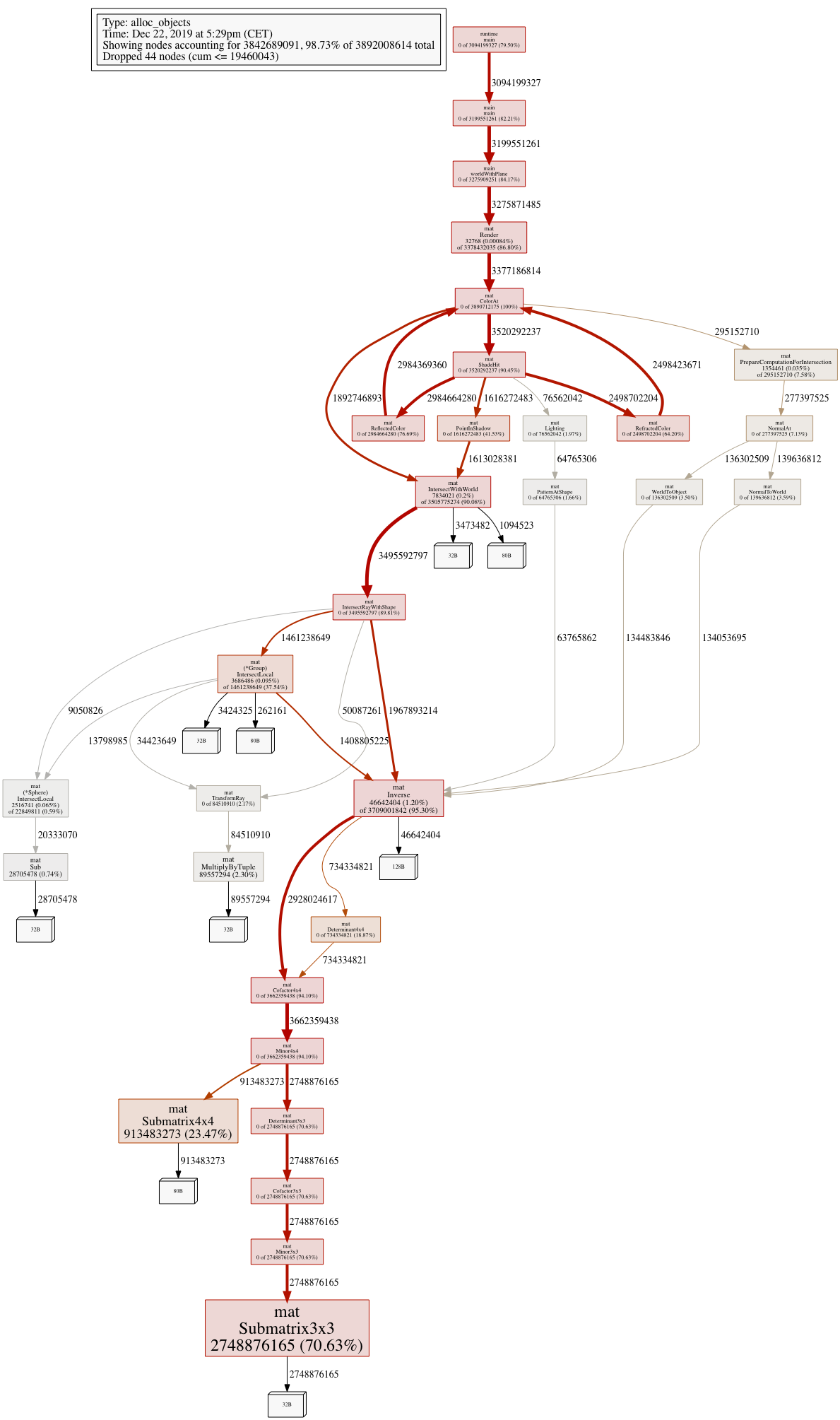
Yes, look at that Inverse() function. Over 95% of all memory allocations are happening in it’s descendants! A closer look:

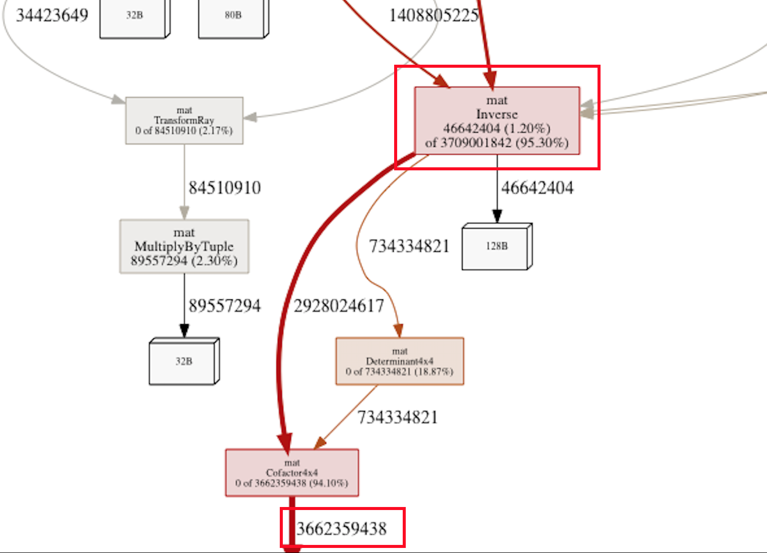
Yup - someone down that call hierarchy is performing about 3.7 billion(!) allocations for rendering a 640x480 image!! That’s more than 12000 allocations per pixel being rendered. Something was definitely rotten in my own little kingdom of ray-tracing.

4.1 Caching the inverse transformation matrix

While “inverse the transformation matrix” sounds like something Picard could say in Star Trek, it’s one of those fundamental pieces of math that our ray-tracer needs to happen when moving from “world space” to “object space” when performing a ray intersection test on an object. Since we’re testing all objects in the scene on every ray being cast, including reflections and shadows, this adds up to an enormous amount of matrix math that needs to happen.

(The transformation matrix is a 4x4 matrix that keeps track of the translation (position in 3D space), rotation and scaling of our primitives in relation to the “world” cartesian coordinate system.)

The good news is that we actually needed to calculate the inverse transformation matrix for our scene objects exactly once. So once we know where in world space our camera and scene objects are, we can calculate their inverse transformation matrices once and store the result in their structs:

type Sphere struct {
	Transform        Mat4x4  // Store Transformation matrix here
	Inverse          Mat4x4  // Store the Inverse of the above here
}
// SetTransform multiplies the current transformation matrix with the passed transform and stores the result.
// The new inverse is also calculated and stored.
// Should only be called during scene setup.
func (s *Sphere) SetTransform(translation Mat4x4) {
	s.Transform = Multiply(s.Transform, translation)
	s.Inverse = Inverse(s.Transform)
}
func (s *Sphere) GetTransform() Mat4x4 {
	return s.Transform
}
func (s *Sphere) GetInverse() Mat4x4 {
	return s.Inverse
}

In practice, SetTransform(translation Mat4x4) above is only called once when we’re setting up the scene.

This was a trivial optimization to code, but it made a huge difference: The time needed to render the reference image went from 1m30 to about 4.5 seconds!! A single threaded render went from 3m15s to about 10s.

Looking at allocations, we went from 3.8 billion allocations to “just” 180 million and the total amount of memory allocated went from 154 GB to 5.9 GB. While we certainly saved a significant number of CPU cycles for the actual math of calculating the inverse, the big part of this optimization definitely was easing the pressure on the memory subsystem and the garbage collector since calculating the inverse required allocating memory on each invocation. The Inverse() function is now used so sparingly it doesn’t even show up when doing a heap profile.

5. Reducing allocations & Caching

3.7 billion down, 180 million to go? If I had the time and will (which I don’t) I’d probably rewrite everything from scratch with a “zero-allocation” goal in mind. Keep things on the stack, pre-allocate every piece of memory needed to hold results, check inlining etc.

I should perhaps mention that when I begun implementing things based on the book, I used a “everything should be immutable” architecture. While that did really help with correctness and avoiding nasty bugs due to (accidental) mutation, allocating new slices or structs on every single computation turned out to be a quite horrible idea from a performance point of view.

Since I didn’t want to start over (and have to refactor at least a hundred implementations of those cucumber tests implemented in plain Go), I took an approach of trying to identify one big “allocator” at a time in order to see if I could make it re-use memory or keep its allocations on the stack. Heap profiler to the rescue!

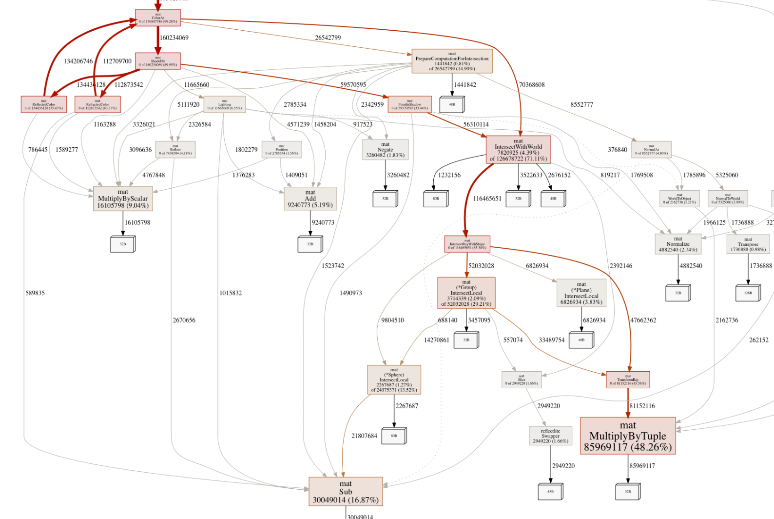
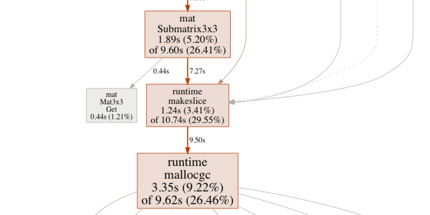
Looking at this new heap profile, the biggest culprit seems to be this MultiplyByTuple function responsible for almost 50% of the remaining allocations. It’s a quite central part of the ray-object intersection code so it’s being called often. What does it do?

func MultiplyByTuple(m1 Mat4x4, t Tuple4) Tuple4 {
	t1 := NewTuple()
	for row := 0; row < 4; row++ {
		a := m1[(row*4)+0] * t[0]
		b := m1[(row*4)+1] * t[1]
		c := m1[(row*4)+2] * t[2]
		d := m1[(row*4)+3] * t[3]
		t1[row] = a + b + c + d
	}
	return t1
}

Yes, it’s just a simple function that multiplies a 4x4 matrix with a 1x4 tuple and returns the resulting tuple. The problem is the NewTuple:

type Tuple4 []float64

func NewTuple() Tuple4 {
	return []float64{0,0,0,0}
}

Oops. It’s creating a new slice on every invocation. That’s not always desirable in a performance-critical context. (In a later part I’ll return to the question of “slices vs arrays”.)

What we would like to do is to have the calling code pass a pointer to a struct in which we can store the result, and hopefully the calling code can reuse the allocated memory or keep it on the stack.

func MultiplyByTuplePtr(m1 Mat4x4, t Tuple4, out *Tuple4) {
    for row := 0; row < 4; row++ {
	out[row] = (m1[(row*4)+0] * t[0]) +
		(m1[(row*4)+1] * t[1]) +
		(m1[(row*4)+2] * t[2]) +
		(m1[(row*4)+3] * t[3])
}

Easy peasy - a new third parameter passes a pointer to a Tuple4 and we’re down to zero allocations. However, there’s a bit more to it. The most typical usage is in this code:

func TransformRay(r Ray, m1 Mat4x4) Ray {
	origin := MultiplyByTuple(m1, r.Origin)
	direction := MultiplyByTuple(m1, r.Direction)
	return NewRay(origin, direction)
}

In this snippet, we’re creating a new transformed Ray (a ray is a point in 3D space and a vector holding its direction) from a matrix and another ray. The results are then put into the new Ray. Moving the NewTuple() call here won’t help us at all. No, this requires a bit more refactoring so the whole call chain uses the C-style pattern of passing the result as a pointer.

func TransformRayPtr(r Ray, m1 Mat4x4, out *Ray) {
	MultiplyByTuplePtr(&m1, &r.Origin, &out.Origin)
	MultiplyByTuplePtr(&m1, &r.Direction, &out.Direction)
}

This implementation passes pointers to the underlying Tuple4 directly to the MultiplyByTuplePtr, which stores the results directly in the passed Ray pointer. As long as the code calling TransformRayPtr has allocated out *Ray in a sensible way, we’ve probably been able to cut down the number of allocations in a really significant way. The Ray in this case is something that can be safely allocated once per render context recursion and can be pre-allocated.

I won’t go into the exact details on how pre-allocating memory for that Ray works, but on a high level each render goroutine has this “render context” mentioned before, and each render context only deals with a single pixel at a time. The final color of a single pixel depends on many things, in particular the number of extra raycasts that needs to happen to follow reflections, refractions and testing if the point in space is being illuminated. Luckily, we can treat each new “bounce” as a new ray so as long as we have allocated enough “rays” in the context to support our maximum recursion depth, we’re fine with this approach.

We can also use Go’s built-in support for microbenchmarking. Consider these two benchmarks:

// Old way
func BenchmarkTransformRay(b *testing.B) {
	r := NewRay(NewPoint(1, 2, 3), NewVector(0, 1, 0))
	m1 := Translate(3, 4, 5)
	var r2 Ray
	for i := 0; i < b.N; i++ {
		r2 = TransformRay(r, m1)
	}
	fmt.Printf("%v\n", r2)
}

// New way
func BenchmarkTransformRayPtr(b *testing.B) {
	r := NewRay(NewPoint(1, 2, 3), NewVector(0, 1, 0))
	m1 := Translate(3, 4, 5)
	var r2 Ray
	for i := 0; i < b.N; i++ {
		TransformRayPtr(r, m1, &r2)
	}
	fmt.Printf("%v\n", r2)
}

Output:

BenchmarkTransformRay-8 
21970136	        52.3 ns/op

BenchmarkTransformRayPtr-8
54195826	        22.1 ns/op

In this microbenchmark, the latter is more than twice as fast. (Go tip: remember that we should do something with the result, otherwise the Go compiler may optimize away the function call we’re benchmarking altogether.)

5.1 Cache, pre-allocate, cache, pre-allocate…

The results obtained in this section clearly indicated that in order to improve efficiency through reuse of memory, pre-allocating data structures and reusing them and caching things whenever possible was a key component.

A few more examples where pre-allocating memory gave really nice benefits:

5.1.1 Intersection lists

There’s a lot of intersection lists to keep track of “hits” when casting rays through a scene. It turned out that the intersection code for each primitive (e.g. sphere, plane, cylinder, box, triangle etc) was creating a new []Intersection slice on each invocation:

func (p *Plane) IntersectLocal(ray Ray) []Intersection {
	if math.Abs(ray.Direction.Get(1)) < Epsilon {
		return []Intersection{}
	}
	t := -ray.Origin.Get(1) / ray.Direction.Get(1)
	return []Intersection{ // CREATING NEW SLICE HERE. BAD!
		{T: t, S: p},
	}
}

This is the intersection code for a Plane. Note how a fresh slice is created and populated at the end of the method if there were an intersection. This pattern repeats itself for all primitive types.

However, for each render context we also know that once we have “used” the intersection(s) of a given primitive, we can safely re-use the same slice for that primitive for any subsequent ray / primitive intersection test. Therefore, a simple pre-allocated slice of sufficient length on the primitive created a large saving in allocations:

func NewPlane() *Plane {
	return &Plane{
		Transform:        New4x4(),
		Inverse:          New4x4(),
		Material:         NewDefaultMaterial(),
		savedXs:          make([]Intersection, 1), // PRE-ALLOCATED!
	}
}
func (p *Plane) IntersectLocal(ray Ray) []Intersection {
	if math.Abs(ray.Direction.Get(1)) < Epsilon {
		return nil
	}
	t := -ray.Origin.Get(1) / ray.Direction.Get(1)
	p.savedXs[0].T = t   // Note re-use of same slice element.
	p.savedXs[0].S = p   // (a plane have no thickness so it cannot be intersected more than once per ray)
	return p.savedXs
}

Why a slice of size 1? A plane can only be intersected exactly once by a ray. Other primitive shapes may have more intersects by a ray. A sphere may be intersected twice (entry and exit), while cones are worst with up to 4 possible intersections.

Another nice optimization was to look at the top-level render context - what was being created anew for each new pixel being rendered? A lot, it turned out. In its final form, these were things we could pre-allocate and re-use:

type Context struct {
	// ... other stuff omitted ... //

	// pre-allocated structs for various stuff used for first ray cast for a pixel
	pointInView     mat.Tuple4
	pixel           mat.Tuple4
	origin          mat.Tuple4
	direction       mat.Tuple4
	subVec          mat.Tuple4
	shadowDirection mat.Tuple4
	firstRay mat.Ray

	// each renderContext needs to pre-allocate shade-data for sufficient number of recursions
	cStack []ShadeData

	// alloc memory for each sample of a given pixel (when multisampling)
	samples []mat.Tuple4
}

Each ShadeData contains pre-allocated structs needed for a single recursion.. I won’t go into more implementation details, but as one can see there’s quite a few of these “pre-allocated” structs or slices and the complexity of the solution did indeed become significant once I realized how the recursive nature of the ray-tracer affected things.

There’s more of these, but in order to not make this section even longer, the key take-away is that while immutability is a really nice thing to strive for in general computer programs - for really performance critical software, re-using memory, caching and avoiding allocations might be a good thing…

5.1.2 Re-use slice memory

This is a simple one. Many intersection lists were being re-used after a while by explicitly setting them to nil or even doing make on them again (which strictly speaking, isn’t reusing anything other than the variable name…).

Instead, slicing a slice to zero length retains the memory previously allocated for its contents, but allows adding items to it from its 0 index again:

slice = nil       // setting slice to nil basically creates a new empty slice, so the underlying 
                  // memory is released and new memory will be allocated once new items are added.

slice = slice[:0] // reslice. From a usage point of view, the slice is now empty, but the previous 
                  // items in it are still in-memory - but inaccessible. They will be overwritten (in memory)
                  // when new items are added. As long as you don't use the unsafe package, you cannot accidently
                  // access items from before the re-slice. This also means that the slice won't have to
                  // grow unless you're adding more items than in its previous incarnation.

5.2 Outcome of reducing allocations & caching

The changes described above was just a few examples of many optimizations where allocations in computational functions was replaced by letting the caller pass a pointer to the result, memory was pre-allocated and slice-memory was being reused. In the end, the results was approximately the following:

• Duration dropped from ~4.5 to ~1.9 seconds
• Allocation count dropped from 180 million to about 33 million
• Total memory allocated went from 5.9 GB to about 1.3 GB

6. Conclusion

This sums up the first part of this 2-part blog series on my adventures optimizing my little ray-tracer. In the next and final part, I’ll continue with more optimizations.

Feel free to share this blog post using your favorite social media platform! There should be a few icons below to get you started.