Optimizing a simple ray-tracer written in Go, part 2

11 July 2020 // Erik Lupander

This is the second part of my mini-series on how I used the go profiling and built-in benchmarking tools to optimize a naive ray-tracer written in Go. For part 1, click here.

Contents

1. Sorting efficiently
2. Slices vs Arrays
3. Pointers or values?
4. AVX2 using c2goasm
5. A final word on threading
6. Conclusion

(Note: Most of this blog post was written based on using Go 1.13)

This part takes off directly after part 1.

Source code

The full source code for my little ray-tracer can be found here: https://github.com/eriklupander/rt

1. Sorting efficiently

Once I had gotten past all those pre-allocations in section 5 in part 1, I was starting to run out of low-hanging fruit to optimize. A new heap profile to the rescue!

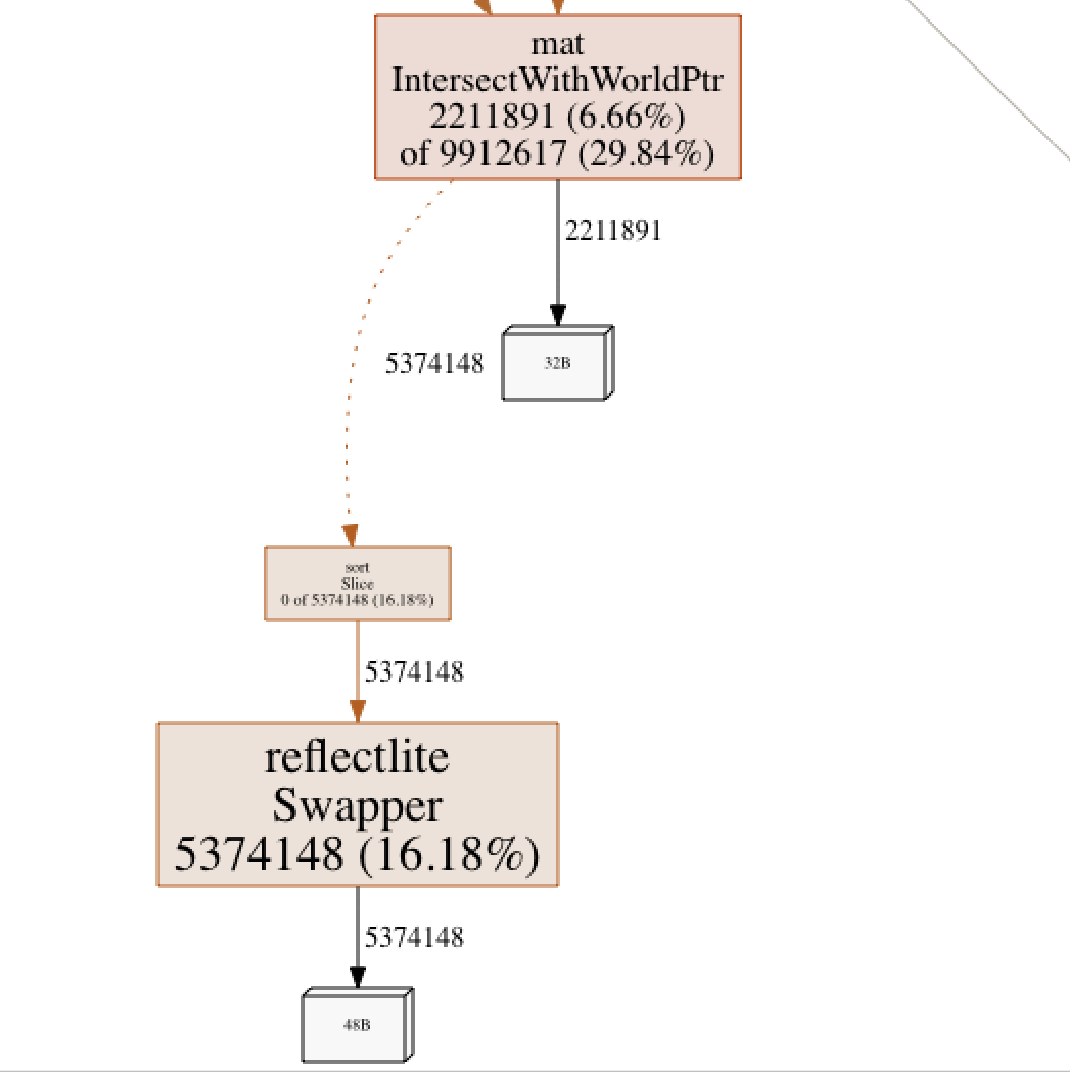
That reflectlite.Swapper needed closer examination. The ray-tracing code sometimes must sort things, intersections in particular. Order of intersections can be important for things like refraction (how light changes direction when entering and exiting various materials). Therefore, every time I had found the intersections of a Ray, I sorted them using sort.Slice:

    // psuedo-code, not actual code from the ray-tracer
    intersections := FindIntersections(world, ray)
    slice.Sort(intersections, func(i, j int) {
        return intersections[i].T < intersections[j].T
    })

As seen above, at this point, sorting accounted for about 16% of all allocations. The quick-fix was to switch to using sort.Sort which requires implementation of the sort.Interface interface:

type Interface interface {
	Len() int
	Less(i, j int) bool
	Swap(i, j int)
}

This required creating a new type for []Intersection that implemented this interface:

type Intersections []Intersection

func (xs Intersections) Len() int           { return len(xs) }
func (xs Intersections) Less(i, j int) bool { return xs[i].T < xs[j].T }
func (xs Intersections) Swap(i, j int)      { xs[i], xs[j] = xs[j], xs[i] }

I then just had to change a few method signatures to take Intersections instead of []Intersection and I could use sort.Sort which allocated way less memory.

This improvement reduced the duration from 1.9 seconds to 1.6 seconds and decreased the number of allocations by about 3 million.

2. Slices vs Arrays

Which one is better for representing 4 64-bit floating point values in a naive ray-tracer?

var vector = make([]float64, 4, 4)
var array = [4]float64

I originally implemented my Tuple4 and Mat4x4 structs with slices for the underlying storage. I tried to read up about the performance-related pros- and cons of using slices over arrays, with the verdict often being “a slice is just a pointer to a type, some index and the underlying array” so it’s just as fast.

Well - somewhere in time I decided I needed to test both ways and carefully benchmark both using go bench but mainly by looking at total render time.

I started by refactoring the entire codebase to use arrays as backing storage for Tuple4 and Mat4x4:

Old

type Tuple4 struct {
	Elems []float64
}

New

type Tuple4 [4]float64

func NewTuple() Tuple4 {
	return [4]float64{0, 0, 0, 0}
}

I think one of the largest benefits was that I now indexed directly into the underlying arrays instead of accessing Tuple4 values through either the Elems or through a Get(index int) method in mathematical functions. Here’s a simple example from code that multiplies a row in one matrix by a column in the another:

// OLD
func multiply4x4(m1 Mat4x4, m2 Mat4x4, row int, col int) float64 {
	a0 := m1.Get(row, 0) * m2.Get(0, col)
	a1 := m1.Get(row, 1) * m2.Get(1, col)
	a2 := m1.Get(row, 2) * m2.Get(2, col)
	a3 := m1.Get(row, 3) * m2.Get(3, col)
	return a0 + a1 + a2 + a3
}
// NEW
func multiply4x4(m1 Mat4x4, m2 Mat4x4, row int, col int) float64 {
	a0 := m1[(row*4)+0] * m2[0+col]
	a1 := m1[(row*4)+1] * m2[4+col]
	a2 := m1[(row*4)+2] * m2[8+col]
	a3 := m1[(row*4)+3] * m2[12+col]
	return a0 + a1 + a2 + a3
}

Honestly, I can’t still say for sure exactly why arrays were faster for my particular use-case, but the speed-up turned out to be significant. The thing is, this refactoring affected so much of the code base that microbenchmarking individual functions was not very conclusive.

However - in the end, rendering the reference image went from 1.6 to 1.1 seconds. At this point, getting a ~30% decrease in total render time was very welcome.

3. Pointers or values for parameters?

I also read up a bit on whether one should pass parameters as pointers or values in Go in regard to performance, where the conclusion typically was something akin to “it’s better to pass by value (e.g. copy) up to a certain size of N bytes” - where N seemed to differ a bit but up to a kilobyte should be fine. Well - I had to test this as well.

I started with a really simple microbenchmark for my Tuple4 Add() function:

func AddPtr(t1, t2 Tuple4, out *Tuple4) { // pass inputs as values
	for i := 0; i < 4; i++ {
		out[i] = t1[i] + t2[i]
	}
}
func AddPtr2(t1, t2 *Tuple4, out *Tuple4) { // pass inputs as pointers
	for i := 0; i < 4; i++ {
		out[i] = t1[i] + t2[i]
	}
}

// BENCHMARKS
func BenchmarkAddPtr(b *testing.B) {
	t1 := NewPoint(3, -2, 5)
	t2 := NewVector(-2, 3, 1)
	var out Tuple4
	for i := 0; i < b.N; i++ {
		AddPtr(t1, t2, &out)
	}
	fmt.Printf("%v\n", out)
}
func BenchmarkAddPtr2(b *testing.B) {
	t1 := NewPoint(3, -2, 5)
	t2 := NewVector(-2, 3, 1)
	var out Tuple4
	for i := 0; i < b.N; i++ {
		AddPtr2(&t1, &t2, &out)
	}
	fmt.Printf("%v\n", out)
}

Results:

BenchmarkAddPtr-8
192414643	         6.29 ns/op

BenchmarkAddPtr2-8
204297358	         5.81 ns/op

Certainly not a huge difference, the “pass by pointer” one is about 8% faster in this microbenchmark. Given that a function such as the Add one is used extensively - for example when determining a pixel’s color given its material’s ambient, diffuse and specular components - even a pretty small improvement such as this one can help improve overall performance.

Similarly, a benchmark comparing passing a 4x4 matrix and a 1x4 tuple to a multiply function shows an even more significant improvement using pointers:

BenchmarkMultiplyByTupleUsingValues-8
79611511	        13.8 ns/op
BenchmarkMultiplyByTupleUsingPointers-8
100000000	        10.7 ns/op

I implemented this change in some critical code paths in the codebase and got a decent speedup.

New duration was 0.8s compared to 1.1s before. Allocations did not change.

4 Using C2GOASM and SIMD/AVX2

I stumbled upon this excellent article which got me thinking that I perhaps could identify some bottleneck mathematical operation and try to improve its execution speed by taking explicit advantage of the SIMD, AVX and AVX2 CPU extensions available on most modern x86-64 microprocessors. I havn’t been able to determine if the Go compiler itself takes advantage of SIMD/AVX on GOARCH=amd64, but I don’t think so at least for my purposes.

For details on this optimization, please check the article linked above. Here’s a quick summary on how I went about replacing my MultiplyByTuple function with a Plan9 assembly implementation taking full advantage of AVX2 that we can call without the overhead of using CGO.

4.1 Intrinsics

Write C code that uses Intel intrinsics in order to perform our Matrix x Tuple multiplication:

void MultiplyMatrixByVec64(double *m, double *vec4, double *result) {
    __m256d vec = _mm256_load_pd(vec4); // load vector into register
    __m256d m1 = _mm256_load_pd(&m[0]); // load each row of the matrix into a register,
    __m256d m2 = _mm256_load_pd(&m[4]); // each register takes 4 64-bit floating point values.
    __m256d m3 = _mm256_load_pd(&m[8]);
    __m256d m4 = _mm256_load_pd(&m[12]);

    __m256d p1 = _mm256_mul_pd(vec, m1); // multiply each row by vector using AVX2
    __m256d p2 = _mm256_mul_pd(vec, m2);
    __m256d p3 = _mm256_mul_pd(vec, m3);
    __m256d p4 = _mm256_mul_pd(vec, m4);

    double d1 = hsum_double_avx(p1); // sum each vector using AVX2
    double d2 = hsum_double_avx(p2);
    double d3 = hsum_double_avx(p3);
    double d4 = hsum_double_avx(p4);

    _mm256_storeu_pd(result, _mm256_set_pd( d4,d3,d2,d1)); // and return a vec4, note opposite order
}

// summing taken from https://stackoverflow.com/questions/49941645/get-sum-of-values-stored-in-m256d-with-sse-avx
inline
double hsum_double_avx(__m256d v) {
    __m128d vlow  = _mm256_castpd256_pd128(v);
    __m128d vhigh = _mm256_extractf128_pd(v, 1); // high 128
            vlow  = _mm_add_pd(vlow, vhigh);     // reduce down to 128

    __m128d high64 = _mm_unpackhi_pd(vlow, vlow);
    return  _mm_cvtsd_f64(_mm_add_sd(vlow, high64));  // reduce to scalar
}

It’s OK if all that C code doesn’t make sense. Note that double equals our Go float64 and that we use _pd intrinsic function variants for double precision. Comments may provide some insight.

4.2 Compile to X86 assembly

Once we had the C-code above ready - one could imagine we’d use CGO to call it, but that’s one of the neat things about this approach - by generating native Plan9 Go assembly, we can basically eliminate the CGO function call overhead. In order to transform this C code into native Go assembly, we first must compile the code into standard x86-64 assembly code using the clang compiler:

clang -S -mavx2 -mfma -masm=intel -mno-red-zone -mstackrealign -mllvm -inline-threshold=1000 -fno-asynchronous-unwind-tables -fno-exceptions -fno-rtti -c -O3 cfiles/MultiplyMatrixByVec64.c

This generates a MultiplyMatrixByVec64.s x86 assembly file.

4.3 Convert to Plan9 assembly

Next, we turn to c2goasm for generating Go Plan9 assembly callable from a .go file.

c2goasm -a -f cfiles/MultiplyMatrixByVec64.s internal/pkg/mat/MultiplyMatrixByVec64_amd64.s

The resulting MultiplyMatrixByVec64_amd64.s contains our Go Plan9 assembly and looks like this (slightly truncated for brevity):

TEXT ·__MultiplyMatrixByVec64(SB), $0-24

	MOVQ m+0(FP), DI
	MOVQ vec4+8(FP), SI
	MOVQ result+16(FP), DX

	LONG $0x0610fdc5               // vmovupd    ymm0, yword [rsi]
	LONG $0x0f59fdc5               // vmulpd    ymm1, ymm0, yword [rdi]
	LONG $0x5759fdc5; BYTE $0x20   // vmulpd    ymm2, ymm0, yword [rdi + 32]
	LONG $0x5f59fdc5; BYTE $0x40   // vmulpd    ymm3, ymm0, yword [rdi + 64]
    ... rest omitted ...

4.4 Making it callable

Finally, we need some hand-written plain Go-code to glue the assembly in MultiplyMatrixByVec64_amd64.s to our ordinary Go code:

//+build !noasm
//+build !appengine

package mat

import "unsafe"

//go:noescape
func __MultiplyMatrixByVec64(m, vec4, result unsafe.Pointer)  // func header matching .s file

func MultiplyByTuplePtr(m *Mat4x4, vec4 *Tuple4, result *Tuple4) { // ordinary go function
	__MultiplyMatrixByVec64(unsafe.Pointer(m), unsafe.Pointer(vec4), unsafe.Pointer(result)) // use unsafe.Pointer to pass args
}

Once here, we can call MultiplyByTuplePtr(m *Mat4x4, f2 *Tuple4, _f4 *Tuple4) just like any other Go code.

4.5 Results

So, how much faster is this code compared to our vanilla MultiplyByTupleUsingPointers we benchmarked previously? A new microbenchmark tells us this:

func BenchmarkMultiplyByTuplePtr(b *testing.B) {
	m := NewMat4x4([]float64{1, 2, 3, 4, 5.5, 6.5, 7.5, 8.5, 9, 10, 11, 12, 13.5, 14.5, 15.5, 16.5})
	t := NewTupleOf(3,5,9,6)
	var out Tuple4
	for i := 0; i < b.N; i++ {
		MultiplyByTuplePtr(&m, &t, &out) // <-- here we call the plan9 assembly through the glue func
	}
	fmt.Printf("%v\n", out)
}

Result (including the previous benchmarks from section 3):

BenchmarkMultiplyByTupleUsingValues-8
79611511	        13.8 ns/op
BenchmarkMultiplyByTupleUsingPointers-8
100000000	        10.7 ns/op
BenchmarkMultiplyByTuplePtr-8         NEW ONE USING AVX2!
232738142	         5.14 ns/op

More than twice as fast! Given that MultiplyByTuple is called several times on every ray / shape intersection test, this fix should definitely provide a nice speedup:

Rendering the reference image now took 0.6s compared to 0.8s before.

I’ve also played around with implementing the Dot and Cross product functions using the same approach. Dot turned out to be significantly slower when done using intrinsics, while Cross was interesting. The microbenchmark showed the intrinsics version to be maybe 15% slower than the pure Go one, but a real render of an image was actually a few percent faster when the Plan9 assembly verison Cross product was used. If anything, it serves as a good reminder that one should be careful drawing conclusions from microbenchmarking isolated functions - the performance of the program as a whole is the most important metric to look at when chasing optimizations.

5. A final word on threading…

With the assembler optimizations above done, I was more or less “done” with my optimizations. However, the topic of multi-threading performance in the ray-tracer remained somewhat of a mystery to me. We saw that the initial improvement (before all other improvements) was about 2.5x. How does multi-threading work out after all other optimizations?

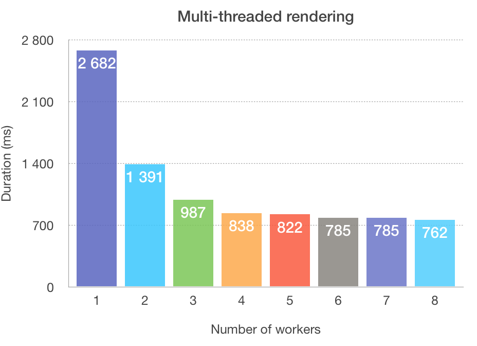
(note that the image rendered for this particular chart isn’t exactly identical to the reference one)

About 3.5x faster using all available 8 thread/workers compared to a single worker. But one must note that there’s very little improvement once we move past 4 threads on my machine.

I havn’t figured this one out exactly, but I believe it boils down to a number of things:

1. Having a CPU (my Mac uses a 4870HQ) with 4 cores / 8 hardware threads (using hyperthreading) doesn’t necessarily mean one should expect the raw performance of 8 “real” CPU cores. Some resources (CPU caches etc) are probably shared within a single core.
2. Memory bandwidth? We’re still allocating and de-allocating a substantial amount of memory. Perhaps the memory subsystem is holding the CPU back?
3. I’ve spent next to no effort actually thinking about efficient multi-threading or optimizations on the CPU-level. I.e. things like optimizing for CPU cache size. In other words - my implementation could very well be a bad one as far as efficient multi-threading is concerned.

I’ve also run the ray-tracer on a more modern Intel Core i9 8 core / 16 thread MacBook Pro 2019 and on a desktop computer with an AMD Ryzen 2600X 6 core / 12 thread CPU, seeing similar behaviour where performance improvements are negligible after worker count > num of physical cores. However, I do remember running the ray-tracer on my Ryzen 2600X with the memory clocked to 2100 Mhz instead of the normal 3200 Mhz. I did notice that the CPU usage was down to 60-70% per core instead of the >99% I saw with the memory at its normal speed, which could indicate memory bandwidth or latency being a culprit. Perhaps I’ll do a follow up on this particular topic!

I’m sure there’s someone out there who could shed some light on this issue. Feel free to use the comments!

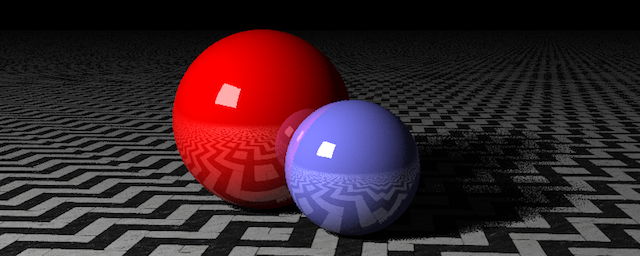
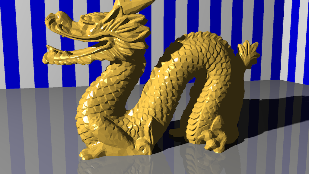
After all these optimizations (+BVHs), rendering a complex scene with tens of thousand of triangles, multi-sampling, soft shadows etc had become possible in reasonable amounts of time. This 1920x1080 render of a dragon took about 20 minutes:

6. Conclusion

First a little reminder that the findings in this blog post are strictly anecdotal and specific to my use case - the naive ray-tracer originally written without performance in mind. Your mileage in other circumstances may vary!

I’m also well aware there’s a lot more one can do such as more comprehensive escape analysis and making sure the compiler inlines function calls properly. That said, going from 3m15s to 0.6s for the exact same result was very rewarding and I learned a ton of stuff doing it. As a bonus, I probably had just as fun doing these performance optimizations as I originally had creating the ray-tracer based on the mentioned “The Ray Tracer Challenge” book.

To give an overview of this optimization journey, the following diagram gives a pretty good view:

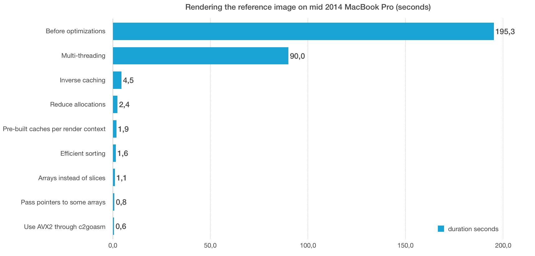
Clearly, the single most important fix was caching the Inverse, probably followed by multi-threading and generally avoiding re-allocating structs and slices in the renderer. The performance gains from slices vs arrays, pointers vs values and sorting were not as clear, but together they did indeed provide a substantial gain. The intrinsics and Plan9 assembly was perhaps stretching things a bit, but nonetheless a fun thing to experiment with.

That’s it! Hope you enjoyed reading my ramblings on ray-tracer performance optimizations in Go.

Feel free to share this blog post using your favorite social media platform! There should be a few icons below to get you started.