Energy blog series, part 4 - EV charger availability.

27 October 2021 // Erik Lupander

This is the fourth part of a blog-series about using CDK and AWS services to build and deploy solutions related to personal energy usage and electric vehicle charging. This part deals with using data from chargefinder.com’s APIs and InfluxDB Cloud in order to be able to forecast DC fast-charger availability at certain charging sites and time of day on common travelling dates.

• 1. The EV charging problem
• 2. Calling ChargeFinder
• 3. The InfluxDB flux query language
• 4. Writing data to InfluxDB Cloud
• 5. Deployment
• 6. Summary

The full CDK and Go source code for this project can be found here: https://github.com/eriklupander/powertracker

Note: I am in no way affiliated with or working for Influxdata, Chargefinder, AWS or any other company or service provider mentioned in this blog post. I’m only doing this for educational purposes and personal enjoyment.

1. The EV charging problem

I got my first fully electric vehicle about 6 months ago, and I’ve enjoyed travelling parts of southern Sweden this past summer. Among EV drivers, range anxiety has been something of “a thing”, but during the family’s trips this summer our conclusion this far isn’t really that range nor charging speed is the main problem. No, the problem is the scarcity of high-speed DC chargers (non-Tesla) and that charging queues tend to form during busy travelling days. Being able to forecast DC fast-charger availability on a longer trip may very well save both time and reduce frustration in my future travels, so I set out to develop a solution (for personal use) to collect charger availability status from the chargefinder.com API and use InfluxDB Cloud V2 to store charger availability as time-series data and then use their Flux API to perform queries that over time hopefully will let me plan longer trips with regard to the question of:

At which times of day on a given weekday can I expect chargers to be available at a given site?

1.1 The Chargefinder API

There’s various websites and apps that lets you see where there are publicly available EV chargers. I’ve tried quite a few of them and my absolute favorite when it comes to user experience and features is Chargefinder.com. While Chargefinder has no official API, opening the Chrome DevTools while browsing a few charge sites reveals a well-designed API used when querying sites and charger availability.

I picked out a limited number (<20) of sites I’m interested in monitoring over time (Chargefinder tracks thousands of sites across Europe) mainly for potential ski-trips the upcoming winter.

1.2 Architecture

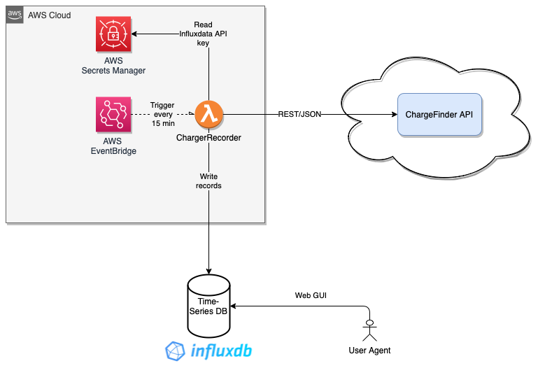
I re-used relevant parts of the Powerexporter lambda solution developed in part 1&2 of this series, with a few key differences:

• The source of data is the Chargefinder REST/JSON API, not the Tibber GraphQL API
• I’m storing queried data in InfluxDB Cloud V2, not AWS TimeStream.

2. Calling ChargeFinder

This part is not that interesting from a technical point of view. I looked up ID’s for the charging sites I wanted to track, and then I use the standard Go http.Client to query them using their REST endpoint, parse the returned JSON etc.

2.1 Call parallelization

The only remotely “special” thing is that I’ve parallelized the ~20 calls and added a timeout to the HTTP calls using context.WithTimeout. The main reason for this is that AWS lambda charges by time spent and sequentially calling this API may very well take over 30 seconds totally.

	// allow max 20 seconds to pass for ALL requests 
	ctx, cfn := context.WithTimeout(context.Background(), time.Second*20)
	defer cfn()

	// encapsulates the http-client used to call ChargeFinder
	chargeFinderProvider := provider.NewChargeFinderProvider()

	// Use a wait-group to wait for all requests to deliver their results.
	wg := sync.WaitGroup{}
	wg.Add(len(chargeFinderSites))
	for _, site := range chargeFinderSites {
		// Let each "collect" run in their own goroutine to make them run in parallell
		go collect(ctx, site, &wg, influxWriter, chargeFinderProvider)
		// add a slight artificial stagger to avoid tripping any potential rate limiters at Chargefinder
		time.Sleep(time.Millisecond * 100)
	}
	wg.Wait()
	logrus.Info("scraping done!")
	influxWriter.Flush()

Using the parallelization above, the total time spent collecting data from ChargeFinder dropped from 20-30 seconds to something like 5-8 seconds depending on how quickly ChargeFinder responds.

2.2 Using jsonparser for response processing

Inside collect the only remotely fancy thing going on is using github.com/buger/jsonparser to iterate over the response body from Chargefinder in order to count the number of available chargers at the time of execution. jsonparser is very fast, but more importantly, it provides an API that lets us iterate over an arbitrary JSON document without resorting to map[string]interface{} and endless type-conversions or having to pre-define a struct for the expected response data. Instead, the jsonparser.ArrayEach allows us to iterate and jsonparser.GetString(value, "id") allows getting a string-typed value for a key attribute on the iteration value.

func parseChargers(ccsChargers []model.CCSCharger, data []byte) (model.Record, error) {
	// variable for keeping track of the number of available chargers
	available := 0
	
	// Use the ArrayEach iterator and an inlined "each" function.
	_, err := jsonparser.ArrayEach(data, func(value []byte, dataType jsonparser.ValueType, offset int, err error) {
		
		// use jsonparser's typed getter to get the "id" field on the entry being processed
		id, _ := jsonparser.GetString(value, "id")
		
		// ccsChargers contains all chargers on the given site, this data comes from metadata fetched elsewhere
		for _, ccsCharger := range ccsChargers {
			
			// If either Identifier or Name matches (don't ask...), check status and if status free, increment 
			// the counter.
			if id == ccsCharger.Identifier || id == ccsCharger.Name {
				status, _ := jsonparser.GetInt(value, "status")
				if status == 2 { // 2 == status free
					available++
				}
				break
			}
		}
	})
	if err != nil {
		return model.Record{}, err
	}
	return model.Record{Available: available, Total: len(ccsChargers)}, nil
}

Of course, there’s more to the ChargeFinder API integration code, but as previously stated, it isn’t terribly interesting, so let’s instead move on to storing the queried data.

3. The InfluxDB flux query language

InfluxDB V2 has a new take on querying time-series data called Flux. Previously, InfluxDB used a SQL-like query-language called InfluxQL. AWS TimeStream - which we’ve used in previous parts of this blog series - also uses a SQL-like query language.

So, what sets Flux apart? The official docs is certainly the best source for this kind of information - but basically Flux adopts functional language programming patterns which makes it much more capable than its predecessor. Features possible with Flux not previously available includes Joins, Pivots, Histograms, flexible Grouping and Sorting. Keep reading for some examples.

3.1 The InfluxDB data model

Before writing data, it’s probably a good idea to take a quick tour of InfluxDB key concepts. If you’re coming from Prometheus or other time-series database, I guess most concepts should feel pretty familiar, but I think a quick primer might be helpful. For example, at a glance - what’s actually the difference between a point and a measurement and how do they apply to each other? What are tags and why are they so important for querying data? And what’s actually a series?

3.1.1 Columns

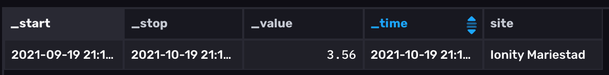
I’ll try a layman’s explanation, starting by looking at a single record of my own data:

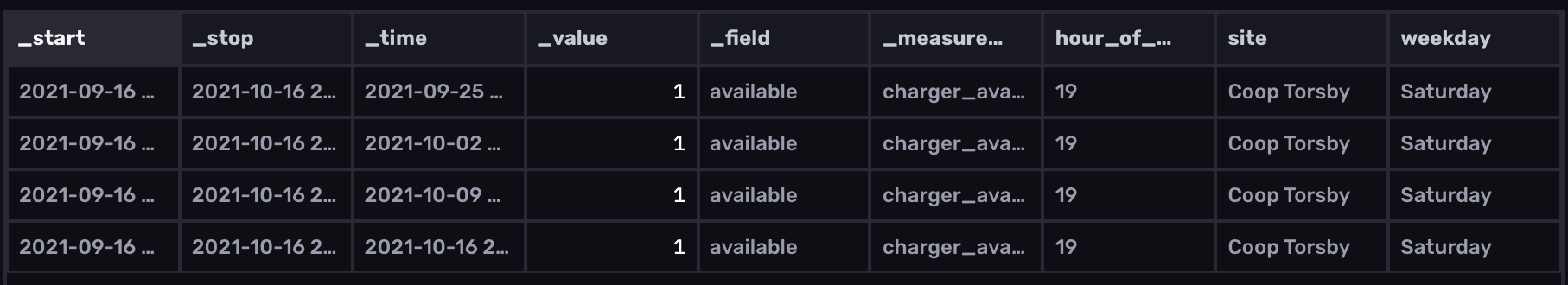
Columns starting with an underscore are defined by InfluxDB / Flux itself:

• start - Starting point in time of the _selected time range of the data points we are looking at. In this case, I had selected to look at data from the past 30 days.
• _stop - See above, the stop time of the time range we’re looking at. Yes, I took that screenshot sometime during the 16th of october 2021. So please note, the _start and _stop columns seen on every data point here does not belong to the actual stored data, it’s an artifact of the query we’ve performed.
• _time - This - on the other hand - is the exact time which the current data point was recorded. The table layout in the screenshot truncates the date, its actual precision is 2021-09-25T04:00:00.000Z. Please note it’s the recording lambda that truncates to the nearest full minute.
• _value - We’re recording the number of available chargers at the given site. There’s only one CCS-charger at Coop Torsby, and it was available when the data point we’re looking at was recorded.
• _field - Ok, now it’s getting a bit more hairy. We’ve got a _field having the label “available”, and next to it we have a _measurement with the value “charger_availability”. What’s the difference? Very simply put - _field is the label for the _value column. And a InfluxDB record can have several fields. I’m just recording a single one, but I could theoretically add a _field for the total number of chargers at the site, and yet other ones that (if the data were available) about how many of the unavailable chargers that were occupied and broken, respectively.
• _measurement - Yeah, what’s the deal here? The measurement column is the label that describes your data. Or as InfluxDB puts it: "A measurement acts as a container for tags, fields, and timestamps.". Our measurement is called “charger_availability”, which provides a bit more context than just that “available” _field.
• hour_of_day - tag for hour of day, 0-23.
• site - tag for name of charging site such as “Ionity Mariestad”
• weekday - tag for day of week. “Monday”, “Tuesday” etc.

Those three last columns are my tags. These tags are defined by me and provides a key-value driven way of giving context and metadata to the entries which can be grouped on, among other useful things. The simplest one in my data is site which is a tag that identifies the charging site the data point belongs to, in this case “Coop Torsby”. The other two should probably be deducible from the _time, but I’m storing them as separate tags for now for easier construction of flux queries to answer questions such as “give me the average availability of Coop Torsby on sundays between 20:00-23:00 over the last 8 weeks:”. We’ll get back to that particular query soon!

3.2 The time series

Now that we’ve gone through some key concepts regarding the different columns, it’s time to start connecting the dots - or points into a series.

So, what’s a series? A series is a collection of data points that shares measurement, tags, and field key(s). The measurement, tags and field key makes up a series key. In my EV dataset, a raw series key could look like this:

charger_availability,site=Ionity Mariestad,weekday=Monday,hour_of_day=15 availability

In my case, I track approx 20 charging sites x 24 hours x 7 days per week. That corresponds to no less than 3360 different time series.

3.2.1 Querying all times series

This query selects all data without any grouping, which should return all time series in my bucket:

from(bucket: "chargerstatus")
  |> range(start: v.timeRangeStart, stop: v.timeRangeStop)
  |> aggregateWindow(every: v.windowPeriod, fn: mean, createEmpty: false)
  |> yield(name: "mean")

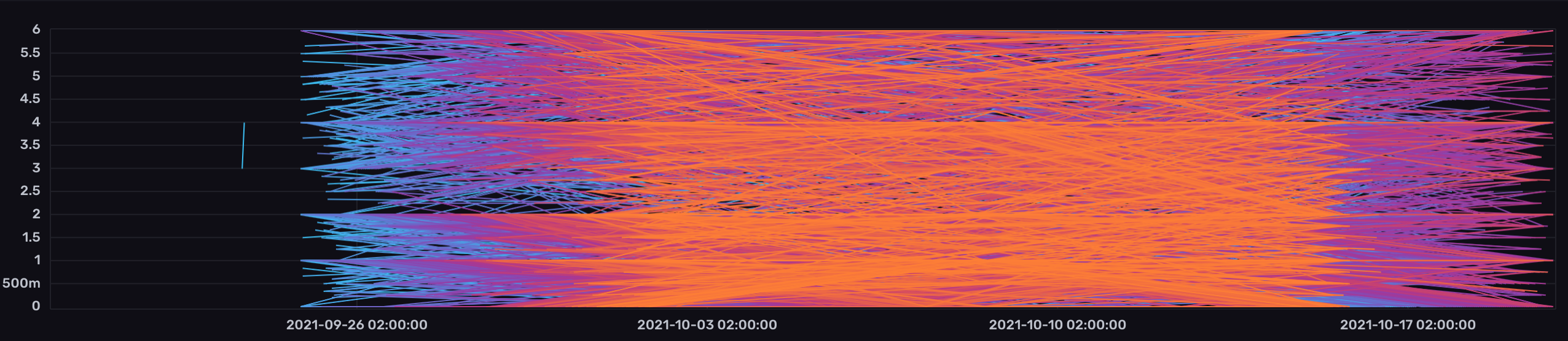
Quite psychedelic. Perhaps a great backdrop for your next rave party. As a useful visualization, not so much.

It’s also known as the problem of “high series cardinality”. Or in short, when your data set has multiple tags with many possible values.

The following image highlights a single time series with some details in the tooltip. This particular time series with the series key charger_availability,site=Ionity Vik (Hönefoss),weekday=Monday,hour_of_day=15 availability contains 4 data points for a given site on Mondays between 15:00-15:59, the highlighted point being on the Monday of 27th of September during which 5.25 chargers on average were available for the data points collected between 15:00-15:59.

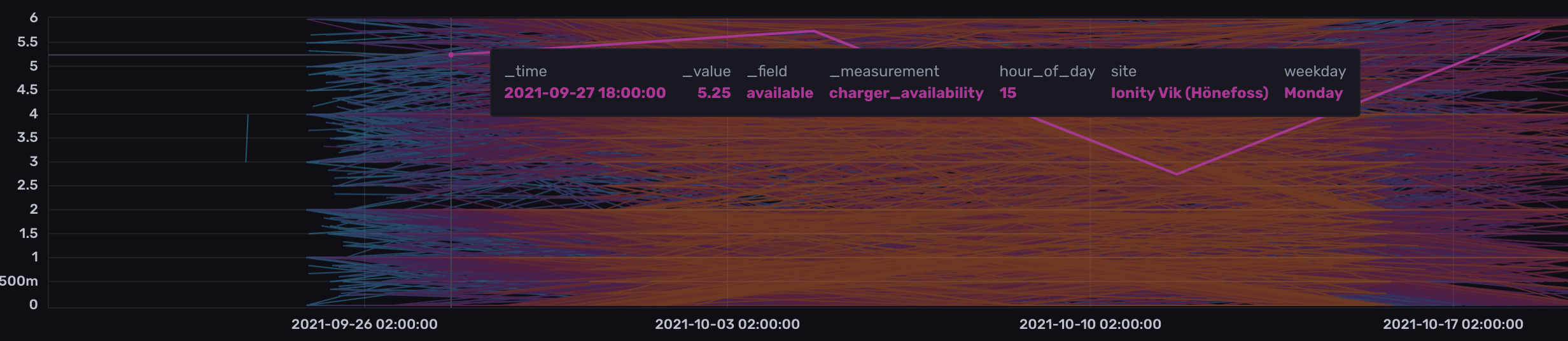
It looks a lot clearer in table form:

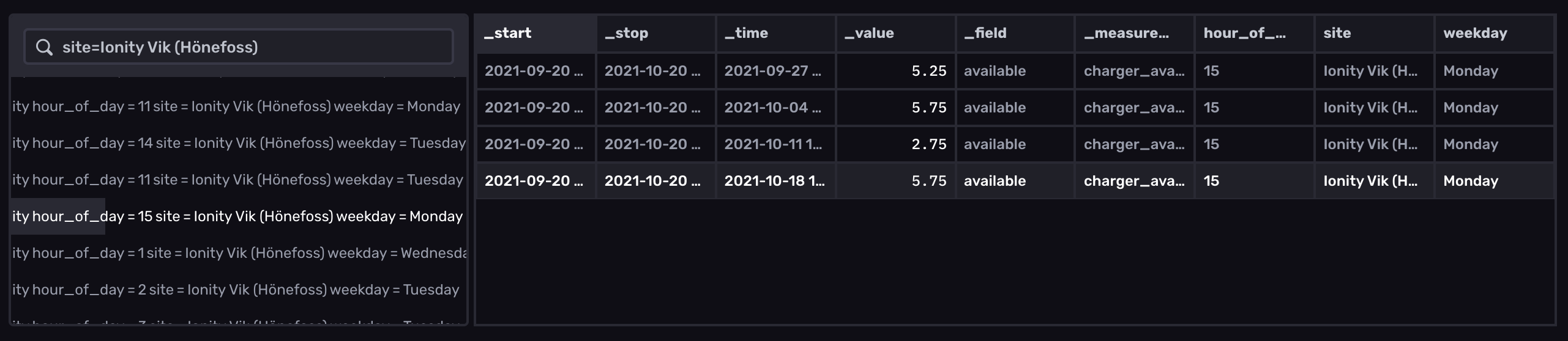
I think this screenshot from the InfluxDB Cloud table view shows how all series returned by the query are listed in the left table - one per series key (or combination of tags) - and then we see the data points of one selected series in the main right-hand table.

3.2.2 Filtering and grouping

We use filter to select columns to include in a query, and we use group to group entries for a given tag. This particular query shows availability between 20-23 on Sundays for Ionity Mariestad on an average across 8 weeks:

from(bucket: "chargerstatus")
  |> range(start: v.timeRangeStart, stop: v.timeRangeStop)
  |> filter(fn: (r) => r["_field"] == "available")
  |> filter(fn: (r) => r["site"] == "Ionity Mariestad")
  |> filter(fn: (r) => r["weekday"] == "Sunday")
  |> filter(fn: (r) => r["hour_of_day"] == "20" or r["hour_of_day"] == "21" or r["hour_of_day"] == "22" or r["hour_of_day"] == "23")
  |> group(columns: ["site"])
  |> aggregateWindow(every: 8w, fn: mean, createEmpty: false)
  |> yield(name: "mean")

Another query that shows the full availability for the same site on a per-record basis, rendered as a graph: (since the ~600 entries in table form wouldn’t make a very compelling blog post)

from(bucket: "chargerstatus")
  |> range(start: v.timeRangeStart, stop: v.timeRangeStop)
  |> filter(fn: (r) => r["_field"] == "available")
  |> filter(fn: (r) => r["site"] == "Ionity Mariestad")
  |> group(columns: ["site"])
  |> aggregateWindow(every: v.windowPeriod, fn: mean, createEmpty: false)
  |> yield(name: "mean")

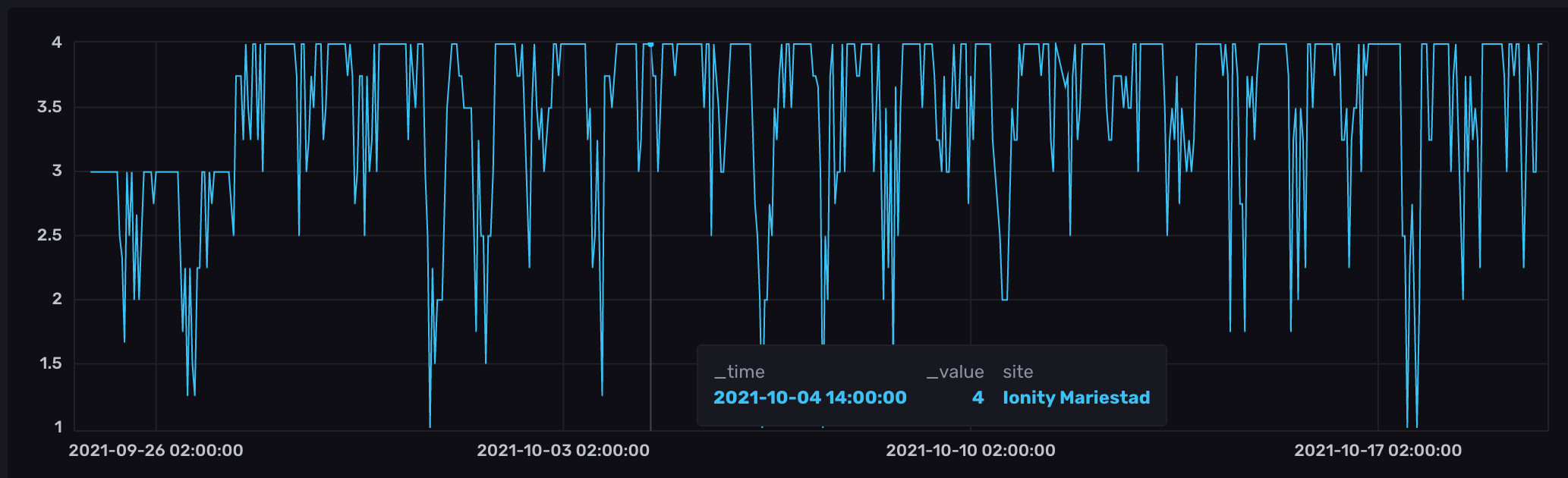
By not filtering on the weekday and hour_of_day tags and using windowPeriod instead of the 8-week aggregate from the query above, we get a single contiguous time series.

I’m just a lowly flux beginner, so there’s probably better ways to accomplish the above - and I’m just scratching the surface of what one can do with Flux - nevertheless, I do think it’s a quite powerful query language for time-series data providing somewhat relational-like capabilities with grouping, aggregation and filtering as well as the more vanilla time-series stuff.

3.3 Cost?

The InfluxDB V2 free tier provides more than enough writes and entries for the purpose of this little hobby project. However, since the max data retention of the free tier is 30 days, I’ve started a paid account in order to keep my data indefinitely.

There’s a blog post detailing how your bill is calculated, based on four discrete pricing vectors:

• Data in
• Data out
• Storage
• Queries

I expect my bill to be very reasonable. My lambdas probably ingest at most a few hundred kilobytes per day, which at $0.002/MB for data in should translate to a few cents per month. Queries are 1 cent per 100 queries, and unless I go really bananas with my querying, I also expect at most a few cents for queries. Data storage will grow over time. I don’t have an exact figure, but I think I’m totally ingesting somewhere between 10-30 mb per month. Let’s say I will average 100 mb until I’m satisfied or start evicting data. Then $0.002/GB-hour translates to 1-2 cents per month. Finally, data out should vary on how much data my queries emit. At $0.09/GB this may very well be the largest cost depending on what kinds of queries I run. However, I don’t expect anything extraordinary here.

All in all - it looks like my costs will be less than $1 per month, possbibly as low as < 10 cents. I’ll get back with an update when a few bills have arrived.

4. Writing data to InfluxDB Cloud

Influxdata has a Go client library that provides a simple and efficient API to use for writing data. When compared to AWS TimeStream Go client code, I do think that the InfluxDB Go API is cleaner and more concise - though apples and oranges might apply!

4.1 Connection setup

To read or write data using the Go client library, one needs to set up a Client which then can be used to create various APIs for reading, writing, deleting operations.

The boilerplate for setting up a Go InfluxDB non-blocking api.WriteAPI is really simple:

func NewInfluxWriter(influxTbToken, bucket, org string) *InfluxWriter {
	client := influxdb2.NewClient("https://eu-central-1-1.aws.cloud2.influxdata.com", influxTbToken)
	return &InfluxWriter{writeApi: client.WriteAPI(org, bucket)}
}

First, the InfluxDB V2 client is set up using endpoint URL and my personal InfluxDB Cloud access token I’ve retrieved from AWS Secrets Manager. Next, an api.Writer is created for a named organization and bucket. These two latter concepts might need a bit of extra explanation:

• organization: This is the account identifier you used when registering your user at InfluxDB Cloud. For example, an email address.
• bucket: The bucket is where your data goes. As an organization, you may have many buckets. In this particular use-case, I use a single bucket called chargerstatus that I created using the InfluxDB Cloud web console.

Time to write som data points!

4.2 Writing data

I’ve wrapped the Go client in my own InfluxWriter struct which exports a single Write method:

func (iw *InfluxWriter) Write(r model.Record) {
	now := time.Now()
    
	p := influxdb2.NewPointWithMeasurement("charger_availability").
		AddTag("site", r.SiteName).
		AddTag("weekday", now.Weekday().String()).
        AddTag("hour_of_day", strconv.Itoa(now.Hour())).
		AddField("available", r.Available).
		SetTime(now)

	iw.writeApi.WritePoint(p)
}

Using the NewPointWithMeasurement constructor function from the influxdb2 package, we can construct a single point using a fluent DSL, providing measurement name, three tags and the field “available” that records the number of available chargers for the given site at the current date and time. Finally, we call WritePoint on our api.Writer to send it to the buffer.

Wait, what buffer? Well - when using the InfluxDB2 asynchronous API, records first goes into a buffer which is flushed when it reaches a certain size (default: 5000) or when it times out (default 1s). Therefore, we should call Flush() when we’re done writing our charger statuses and/or Close the client to make sure there’s no non-flushed entries in the buffer when our lambda exits.

For even more fine-grained control, the Go client library offer more options such as a synchronous API as well as possibility to write entries using the InfluxDB line protocol.

All in all - in my humble opinion, the InfluxDB APIs are well-designed and has been a breeze to work with.

5. Deployment

Just like the lambdas and AWS services deployed in previous installments of this series, I’m using AWS CDK to deploy this new stack as well.

For convenience, I’m keeping the code in the same repo as before, but defined in a new Stack declared alongside the existing Powerrecorder stack, with some code re-use as a bonus.

Here’s the full code:

export class ChargerStatusStack extends cdk.Stack {
    constructor(scope: cdk.Construct, id: string, props?: cdk.StackProps) {
        super(scope, id, props);
        
        // IAM policies, note re-use of tibber_config secret to save some $
        const secretsPolicy = new iam.PolicyStatement({
            actions: ["secretsmanager:GetSecretValue"],
            resources: ["arn:aws:secretsmanager:*:secret:prod/tibber_config-*"]
        })

        // Build lambda that reads data from Chargefinder and stores in InfluxDB cloud
        const chargerStatusFunction = new GolangBuilder(this, "golang builder")
            .buildGolangLambda('chargerStatus', path.join(__dirname, '../functions/statusrecorder'), 60);

        // Build EventBridge rule with cron expression and bind to lambda to trigger chargerStatus lambda
        const rule = new ruleCdk.Rule(this, "collect_charger_status_rule", {
            description: "Invoked every 15 minutes to collect current charger state",
            schedule: Schedule.expression("cron(0/15 * * * ? *)")
        });
        rule.addTarget(new targets.LambdaFunction(chargerStatusFunction))

        // Add IAM for powerrecorder
        chargerStatusFunction.addToRolePolicy(secretsPolicy)
     }
}

One of the improvements is the new GolangBuilder class shared with the other lambdas:

export class GolangBuilder extends Construct {
    buildGolangLambda(id: string, lambdaPath: string, timeout: number): lambda.Function {
        const environment = {
            CGO_ENABLED: '0', GOOS: 'linux', GOARCH: 'amd64',
        };
        return new lambda.Function(this, id, {
            code: lambda.Code.fromAsset(lambdaPath, {
                bundling: {
                    image: lambda.Runtime.GO_1_X.bundlingImage,
                    user: "root",
                    environment,
                    command: [
                        'bash', '-c', [
                            'make lambda-build',
                        ].join(' && ')
                    ]
                }
            }),
            handler: 'main',
            runtime: lambda.Runtime.GO_1_X,
            timeout: cdk.Duration.seconds(timeout),
        });
    }
}

This is IMHO a good example of how powerful the CDK model is, where good DRY principles can be applied to Infrastructure as Code solutions in a programmer-familiar way.

5.2 InfluxDB provisioning?

As far as I know, AWS CDK can’t natively provision any InfluxDB Cloud resources. Note though that there’s an InfluxDB on AWS offering available that might open up some possibilities. Additionally, perhaps it’s possible to let CDK execute some arbitrary typescript code when deploying a Stack, which theoretically could perform InfluxDB Cloud provisioning through the REST API or similar?

6. Summary

To summarize - in this part we’ve developed and deployed a new lambda function that retrieves charger availability and stores the data in InfluxDB Cloud. We’ve also taken a little look at the flux query language for InfluxDB and how to use its powerful grouping and filtering functions to query our time-series data.

I’m quite happy with InfluxDB Cloud and what it offers! A bit of criticism though - since registering approximately 4 weeks ago, I’ve gotten no less than 21(!) unsolicited emails from them ranging from welcome emails to info about upcoming events and new blog posts. I have no problem with a welcome email and perhaps a monthly summary of what’s new and coming up, but these almost daily emails I’d rather opt-in to rather than having to opt-out.

So, how’s charger availability looking? Being both a software craftsman as well as an EV driver, I guess the only possible answer is “it depends”…

On a more serious note, it looks OK-ish. I’m hoping to do a ski trip this winter to Vemdalen, a 680 km drive from Gothenburg:

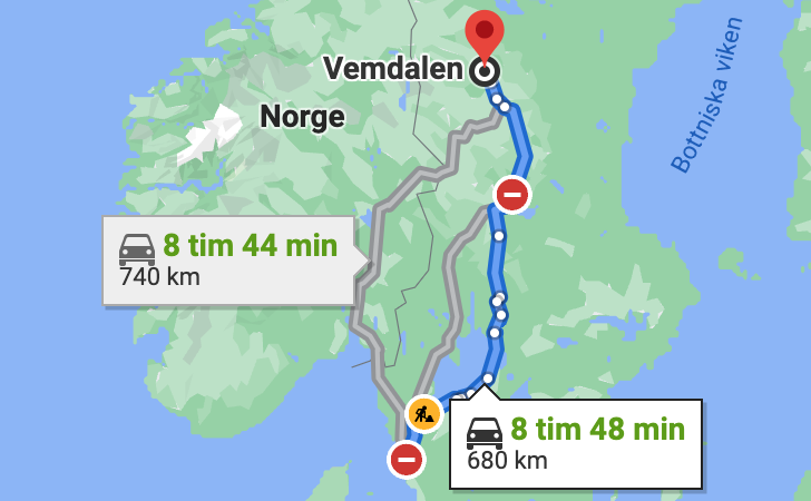
Source: Google Maps

The following query keeps track of the aggregated per 8-hour availability of key chargers along the route:

from(bucket: "chargerstatus")
  |> range(start: v.timeRangeStart, stop: v.timeRangeStop)
  |> filter(fn: (r) => r["_field"] == "available")
  |> filter(fn: (r) => r["site"] == "Bilmetro Noret" or r["site"] == "Handelsområdet Noret" or r["site"] == "Ionity Mariestad" or r["site"] == "McDonalds Kristinehamn" or r["site"] == "Sveg")
  |> group(columns: ["site"])
  |> aggregateWindow(every: 8h, fn: mean, createEmpty: false)
  |> yield(name: "mean")

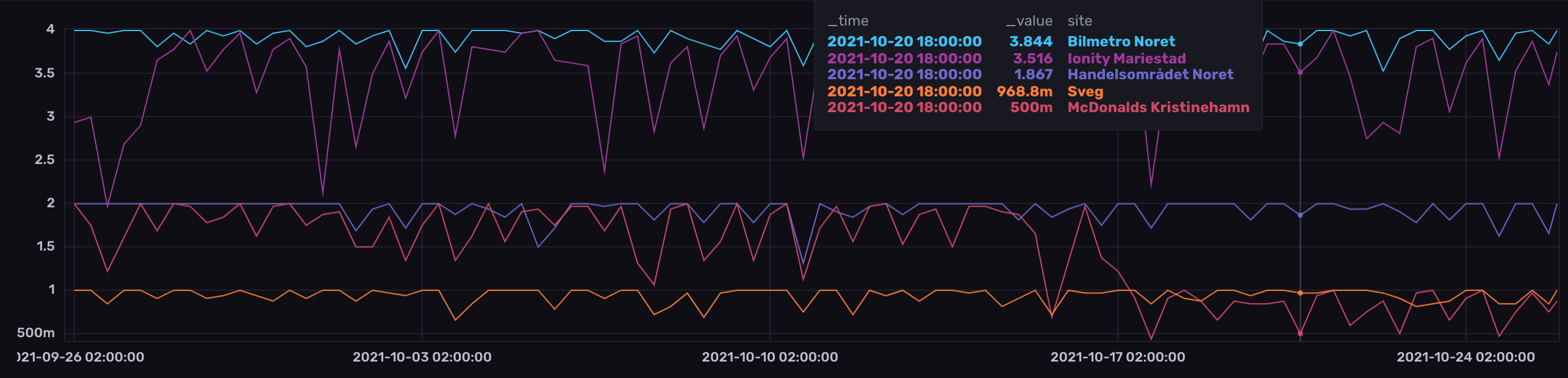
During October, it’s looking good with great availability of the trip-wise very important charger in Mora (Bilmetro Noret), while the two chargers at McDonalds Kristinehamn may be a sore spot - especially given that one of them seems to have gone out of order about 10 days ago without being repaired. However - traffic along this route is quite low in October. Weekends during the skiing season, Mora is a giant traffic jam, so I suspect figures during x-mas break and february school breaks will be very different.

Anyway - this has been a fun exercise and learning some flux has been great!

Until next time,

// Erik Lupander