Blogg
Här finns tekniska artiklar, presentationer och nyheter om arkitektur och systemutveckling. Håll dig uppdaterad, följ oss på LinkedIn
Här finns tekniska artiklar, presentationer och nyheter om arkitektur och systemutveckling. Håll dig uppdaterad, följ oss på LinkedIn

In this part, we’ll take a quick look at OpenCL in general and a bit deeper look at how to make Go play nicely with OpenCL.
Disclaimer: OpenCL is a complex topic, and I’m writing these blog posts mostly as a learning exercise, so please forgive any misconceptions present herein.
If part 1 didn’t get the point across - Path Tracing is really computationally expensive. We want performance, and lots of it.
There’s at least two options one can pursue to improve performance for a math-heavy application such as a path-tracer;
For this blog post, I went with option #2 - utilize the GPU. As API, I picked OpenCL, since I want support for OS X, Windows and Linux - which means Metal is out. I also want to be able to run on both AMD, Nvidia and Intel GPUs, which means CUDA is disqualified. Vulkan seems to be extremely complicated. That leaves OpenCL, which is mature, well documented and there’s CGO-based wrappers available for Go.
Just to make things clear - it’s still going to be a Go program, mostly based on the existing codebase from my old Go-only Path Tracer. The application-level architecture can be described a bit like a frontend/backend solution:
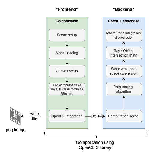
As seen, the “frontend” prepares the “scene” with camera, objects etc. and then the “backend” written in OpenCL will (per pixel) perform the heavy lifting. In more strict OpenCL terms, the “frontend” part is referred to as the “host program”, while the backend part is implemented in an OpenCL C kernel.
That said - let’s not get ahead of ourselves. This blog post won’t contain any path tracing, we’ll just lay down the basics regarding using OpenCL with Go. Let’s start by taking a quick and high-level look at OpenCL.
I’ve created a little repo on github with the examples used in this blog post. They’re strictly Go/OpenCL related, so no fancy path-tracing stuff there!
See: https://github.com/eriklupander/opencl-demo
OpenCL is short for “Open Computing Language”, was initially released back in 2009 by Khronos Group and is (quoting wikipedia):
“a framework for writing programs that execute across heterogeneous platforms consisting of central processing units (CPUs), graphics processing units (GPUs), digital signal processors (DSPs), field-programmable gate arrays (FPGAs) and other processors or hardware accelerators.”
That sounds very nice and dandy, but how does it work from a more practical point of view?
First off - it provides a unified programming model to execute code, regardless whether you want to run the code on your CPU, GPU or even some DSP having OpenCL support. The language traditionally used to write OpenCL kernels (i.e. programs) is C, though some support for C++ exists since 2020.
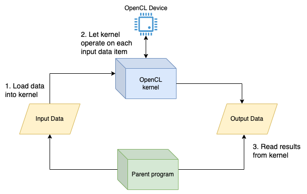
Secondly - I’m going to simplify things a bit in order to explain what OpenCL really does. Look at the following diagram:
Stupid example #1:
Input        Kernel     Output
[1,2,3,4] => square => [1,4,9,16]
A real example of a “square” kernel can look like this:
__kernel void square(
   __global int* input,
   __global int* output)
{
   int i = get_global_id(0);
   output[i] = input1[i] * input1[i];
}
The kernel would be called 4 times, once per work-item, squaring the input by itself, and writing the result to the output. In other words: The code in an OpenCL kernel is an algorithm or operation we want applied to a single work-item.
So yes - basically, we can see an OpenCL kernel as a quite stupid piece of code that’s awesome at executing the same code over and over again for each “input item”, then storing the result in the corresponding “output item”. I think a lot of the magic sauce here is the built-in get_global_id(0) function that returns the index of the input data currently being processed. In this simple example, its just 0,1,2,3 and we’re done after multiplying output[i] = input[i]*input[i]. The neat thing here is that behind the scenes, OpenCL can take advantage of the parallel execution capabilities of CPUs/GPUs and in practice execute all four “invocations” in parallel.
The beauty of OpenCL and “compute” devices is when we scale this up. Let’s say we have a 1920x1080 pixel image we want to lighten up a bit by increasing each pixel’s RGB value by 5%. This time, it’s not 4 invocations, it’s ~2 million if we do it per-pixel. While there’s no GPU in existence(?) that has 2 million “shader units” or “stream processors” (the name varies depending on vendor), high-end GPUs can have several thousand stream processors each capable of executing the “lighten” kernel, so with a correct division of work (i.e. optimize so each stream processor gets an optimal number of pixels to process) it’ll make really short work of the “lighten task”, storing the result in an output buffer.
Read and write buffer (input and output) sizes doesn’t have to be uniform. We could have a “grayscale” kernel that would operate on RGBA float values, 4 per pixel, and return a single float per pixel as its grayscale representation.
There’s a ton of additional complexity one can dive into regarding how to structure input data. I’ll touch on that later. Oh, for the purpose of this blog post, never mind that __global address space qualifier just yet.
Anyway - that was a really short primer.
So, we write OpenCL code in C, but OpenCL programs doesn’t exist in isolation. You always have a host program written in some mainstream language that can call the OpenCL C APIs natively or through a binding layer such as CGO. Of course, one can write the host program in C, but that’s outside my comfort zone, so we’re sticking with Go.
In order to bridge between Go and the OpenCL API, we’re going to use a CGO-based wrapper library for OpenCL 1.2. I do know that this is an archived and rather old fork of an even older repo, for an aging version of OpenCL. Nevertheless, it works just fine for my purposes, so won’t delve any deeper into exactly how the CGO wrapper works etc.
There’s a quite a bit of complexity involved setting up an actual OpenCL context and creating the objects required to execute some code on an OpenCL device, so I think we should take a quick look at the most important building blocks used when creating a simple “Hello world”-like program. We can call it “Hello square”!. It’s a bit like a hierarchy:
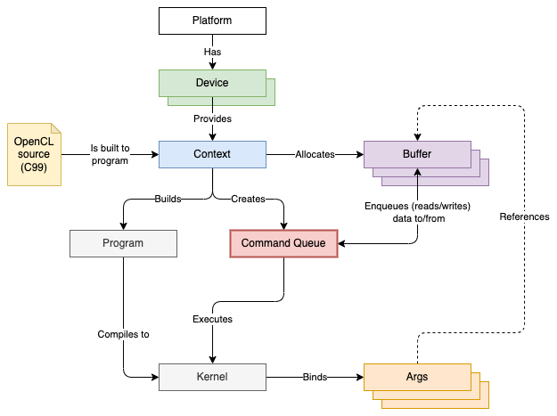
The figure above is slightly simplified, but if read from top to bottom, it sort of converges on that “command queue” that we pass our “input” data to, and which we also use the retrieve the “output” data from.
Name: Apple
Vendor: Apple
Profile: FULL_PROFILE
Version: OpenCL 1.2 (Aug 30 2021 03:51:40)
Extensions: cl_APPLE_SetMemObjectDestructor cl_APPLE_ContextLoggingFunctions cl_APPLE_clut cl_APPLE_query_kernel_names cl_APPLE_gl_sharing cl_khr_gl_event
Devices, where a Device is something that is capable of executing OpenCL code. Typically, a CPU or GPU. There’s a ton of metadata available for each Device describing its capabilities. In practice, I’ve noticed that CPUs work very well, while GPUs such as the Iris iGPU on my old Mac can’t handle my path tracing code, possibly because I’m using a lot of double-precision floating point types.
Device 0 (CPU): Intel(R) Core(TM) i7-4870HQ CPU @ 2.50GHz
Device 1 (GPU): Iris Pro
Device 2 (GPU): GeForce GT 750M
Device and acts as a kind of “factory” to produce the other resources required to create and execute an OpenCL Program.BuildProgram method on the Context.kernel source. Technically, a Program may contain several kernels, but for our purposes, let’s just say one program contains one kernel. A kernel looks like a typical function in mainstream programming languages, having a name and a list of arguments with address space, type and name.
__kernel void square(__global int* input, __global int* output) {
 // code goes here!
}
Device memory through write buffers, starting Kernel execution, and finally reading results back from read buffers.Let’s do a Hello World-like Go program that uses that square Kernel.
Full source: https://github.com/eriklupander/opencl-demo/blob/main/internal/app/square.go
We’ll create main.go and start with obtaining the Platform, Devices and a Context.
Note! A lot of the error-checking has been omitted in the blog post to keep the code more concise.
package main

import "github.com/jgillich/go-opencl/cl"

var squareSrc = `__kernel void square(
   __global int* input,
   __global int* output)
{
   int i = get_global_id(0);
   output[i] = input[i] * input[i];
}`

func main() {
    // First, get hold of a Platform
    platforms, _ := cl.GetPlatforms()

    // Next, get all devices from the first platform. Check so there's at least one device
    devices, _ := platforms[0].GetDevices(cl.DeviceTypeAll)
    if len(devices) == 0 {
        panic("GetDevices returned no devices")
    }

    // Select a device to use. On my mac: 0 == CPU, 1 == Iris GPU, 2 == GeForce 750M GPU
    // Use selected device to create an OpenCL context and make sure we'll release it afterwards
    context, _ := cl.CreateContext([]*cl.Device{devices[0]})
    defer context.Release()
    fmt.Println(devices[0].Name())
}
If we run the snippet above:
$ go run main.go
Intel(R) Core(TM) i7-4870HQ CPU @ 2.50GHz
We see my laptop’s first OpenCL device, the old and trustworthy Core i7 CPU.
Let’s continue with the semi-boring boilerplate
    // Create a "Command Queue" bound to the selected device
    queue, _ := context.CreateCommandQueue(devices[0], 0)
    defer queue.Release()

    // Create an OpenCL "program" from the source code. (squareSrc was declared in the top of the file)
    program, _ := context.CreateProgramWithSource([]string{squareSrc})

    // Build the OpenCL program
    if err := program.BuildProgram(nil, ""); err != nil {
        panic("BuildProgram failed: " + err.Error())
    }

    // Create the actual Kernel with a name, the Kernel is what we call when we want to execute something.
    kernel, err := program.CreateKernel("square")
    if err != nil {
        panic("CreateKernel failed: " + err.Error())
    }
    defer kernel.Release()
Time for something more interesting. First, we’ll prepare a Go slice of numbers we want squared, e.g. 0,1,2...1023, then we’ll move on to the semi-complex topic of how to pass that data over to OpenCL.
    // create a slice of length 1024, with values 0,1,2,3...1023.
    numbers := make([]int32, 1024)
    for i := 0;i<1024;i++ {
        numbers[i] = i
    }
    // Prepare for loading data into Device memory by creating an empty OpenCL buffer (memory) for the input data.
    // Note that we're allocating 4x bytes the size of the "numbers" data since each int32 uses 4 bytes.
    inputBuffer, err := context.CreateEmptyBuffer(cl.MemReadOnly, 4*len(numbers))
    if err != nil {
        panic("CreateBuffer failed for matrices input: " + err.Error())
    }
    defer inputBuffer.Release()

    // Do the same for the output. We'll expect to get int32's back, the same number
    // of items we passed in the input.
    outputBuffer, err := context.CreateEmptyBuffer(cl.MemWriteOnly, 4*len(numbers))
    if err != nil {
        panic("CreateBuffer failed for output: " + err.Error())
    }
    defer outputBuffer.Release()
Note that we haven’t loaded anything into those buffers yet. The input buffer needs to be populated before calling our kernel, and we’ll read the squared numbers from the output buffer at the end of the program.
The cl.MemReadOnly and cl.MemWriteOnly flags tells OpenCL how we expect the buffer to be used by the kernel. A cl.MemReadOnly flag will prohibit kernel-side code from modifying data in that buffer. The opposite, cl.MemWriteOnly tells OpenCL it can’t read from the buffer, only write to it. Hence, our “input” buffer should be cl.MemReadOnly and the “output” buffer should be cl.MemWriteOnly.
    // This is where we pass the "numbers" slice to the command queue by filling the write buffer, e.g. upload the actual data
    // into Device memory. The inputDataPtr is a CGO pointer to the first element of the input, so OpenCL
    // will know from where to begin reading memory into the buffer, while inputDataTotalSize tells OpenCL the length (in bytes)
    // of the data we want to pass. It's 1024 elements x 4 bytes each, but we can also calculate it on the
    // fly using unsafe.Sizeof.
    inputDataPtr := unsafe.Pointer(&numbers[0])
    inputDataTotalSize := int(unsafe.Sizeof(numbers[0])) * len(numbers) // 1024 x 4
    if _, err := queue.EnqueueWriteBuffer(inputBuffer, true, 0, inputDataTotalSize, inputDataPtr, nil); err != nil {
        logrus.Fatalf("EnqueueWriteBuffer failed: %+v", err)
    }
    fmt.Printf("Enqueued %d bytes into the write buffer\n", inputDataTotalSize)

    // Kernel is our program and here we explicitly bind our 2 parameters to it, first the input and
    // then the output. This matches the signature of our OpenCL kernel:
    // __kernel void square(__global int* input, __global int* output)
    if err := kernel.SetArgs(inputBuffer, outputBuffer); err != nil {
        panic("SetKernelArgs failed: " + err.Error())
    }
}
Note how we bind the buffers as args to the kernel, matching the signature of
__kernel void square(__global int* input, __global int* output)
Run the program again:
$ go run main.go
Intel(R) Core(TM) i7-4870HQ CPU @ 2.50GHz
Enqueued 4096 bytes into the write buffer
Time to rumble! We’ll call the arguably cryptically named EnqueueNDRangeKernel(...) function on the queue with a number of semi-confusing arguments which will start the execution:
    // Finally, start work! Enqueue executes the loaded args on the specified kernel.
    if _, err := queue.EnqueueNDRangeKernel(kernel, nil, []int{1024}, nil, nil); err != nil {
        panic("EnqueueNDRangeKernel failed: " + err.Error())
    }

    // Finish() blocks the main goroutine until the OpenCL queue is empty, i.e. all calculations are done.
    // The results have been written to the outputBuffer.
    if err := queue.Finish(); err != nil {
        panic("Finish failed: %" + err.Error())
    }
    fmt.Printf("Took: %v\n", time.Since(st))
This was my least favourite part to write, simply because it’s taken me just too many attempts to wrap my head around these concepts. This topic evolves around that division of work touched on earlier, and also adds address space qualifiers into the mix. I’ll try to use a metaphor:
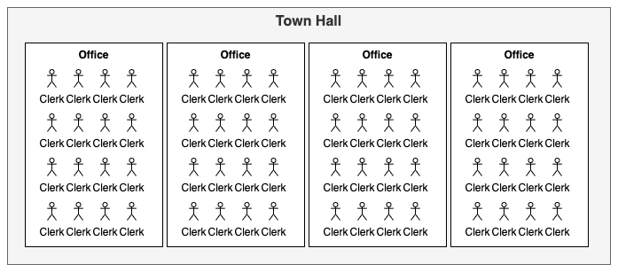
The figure above represents a Town hall, which provides services to members of the community. However, this is a rather uncanny town hall, since all clerks in all offices, can only work on the same task (i.e. kernel) at the same time. Monday’s 8:00-8:30 it’s parking permits, 08:30-11:45 its building permits, 13:00-14:00 its social welfare payouts etc.
To make things even more unsettling, each office within the town hall has the exact same number of clerks.
You’ve probably figured this out by now:
So if we have 4 offices with 16 clerks that all must do the same task, we could process 64 parking permit “kernel executions” at a time. Note that all clerks in the same office must finish their ongoing task before they can start their next batch of work, so if some permit is more difficult to complete than others, that may leave the entire office waiting for a bit for the last clerk to complete. This should make it evident that for optimal throughput, we need to hand out 16 permit applications at a time to each office, otherwise a number of the clerks would just sit idle. This is what we refer to as localWorkSize later.
In OpenCL terms, a modern AMD RX 6900XT GPU with 80 CUs and 64 threads per CU can theoretically execute 5120 kernels in parallell.
Translated to OpenCL, we can for the most part rely on the OpenCL driver to hand out work to available Work groups/Compute units, but we may definitely need to think a bit about how many tasks that are handed to each WorkGroup/CU since that differs between different devices! OpenCL can query a device for its preferred work group size multiple which can give us a hint on which value(s) to pass to EnqueueNDRangeKernel as globalWorkSize and localWorkSize.
Here’s the signature of EnqueueNDRangeKernel which we call to start execution:
EnqueueNDRangeKernel(kernel *Kernel, globalWorkOffset []int, globalWorkSize []int, localWorkSize []int, eventWaitList []*Event) (*Event, error)
This article from Texas Instruments is highly recommended for more details on globalWorkSize and localWorkSize.
This far, we’ve seen the address space qualifier __global. The following 4 qualifiers exists in OpenCL:
Using the City Hall metaphor, global memory is the central hard drive in the basement where everyone gets their “input data” and stores their “output data”. It’s slow! The central hard drive also has a small read-only in-memory RAM disk with constant data everyone can access with lower latencies. Finally, in each office, there’s a local file-server all the clerks can post intermediate results to that can be efficiently shared with the other clerks in the same office/work group. Finally, each clerk has their own tiny little private PDA that offers very limited note-keeping, albeit at the lowest cost in latency.
This far, I’ve primarily used global memory. Parameters declared inside a kernel are implicitly private. Haven’t really used constant or local yet for my purposes.
For more details, I suggest reading the details on these qualifiers elsewhere.
I’ll try to do a layman’s summary below using a simple example:
Given the following 4x4 input (passed as 1D 16-element array):
| 0.000000 | 1.000000 | 2.000000 | 3.000000 |
| 4.000000 | 5.000000 | 6.000000 | 7.000000 |
| 8.000000 | 9.000000 | 10.000000 | 11.000000 |
| 12.000000 | 13.000000 | 14.000000 | 15.000000 |
And the following kernel that returns the square root of the input in each element while logging some details using printf:
__kernel void squareRoot(__global float* input, __global float* output)
{
   int groupId_col = get_group_id(0);  // get id of work group assigned to process "column" dimension
   int groupId_row = get_group_id(1);  // get id of work group assigned to process "row" dimension

   int row = get_global_id(1);         // get row from second dimension
   int col = get_global_id(0);         // get col from first dimension
   int colCount = get_global_size(0);  // get number of columns
   int index = row * colCount + col;   // calculate 1D index
   int localId = get_local_id(0);      // get the local ID, i.e. "thread within the CU"

   // Print (to STDOUT) all values from above to showcase the relationships between workSize, localSize etc.
   printf("row: %d, col: %d, i: %d, local id: %d, groupId_row: %d, groupId_col: %d\n", row, col, index, localId, groupId_row, groupId_col);

   output[index] = sqrt(input[index]); // calculate sqrt given input at index, store result in output at same index.
}
Results in the following output:
| 0.000000 | 1.000000 | 1.414214 | 1.732051 |
| 2.000000 | 2.236068 | 2.449490 | 2.645751 |
| 2.828427 | 3.000000 | 3.162278 | 3.316625 |
| 3.464102 | 3.605551 | 3.741657 | 3.872983 |
We enqueue the data and kernel above using the following arguments:
globalSize := []int{4, 4}
localSize := []int{2, 2}
_, err := queue.EnqueueNDRangeKernel(kernel, nil, globalSize, localSize, nil)
Output from the kernel’s printf statement:
row: 0, col: 2, i: 2,  local id: 0, groupId_row: 0, groupId_col: 1
row: 0, col: 3, i: 3,  local id: 1, groupId_row: 0, groupId_col: 1
row: 1, col: 2, i: 6,  local id: 0, groupId_row: 0, groupId_col: 1
row: 1, col: 3, i: 7,  local id: 1, groupId_row: 0, groupId_col: 1
row: 2, col: 2, i: 10, local id: 0, groupId_row: 1, groupId_col: 1
row: 2, col: 3, i: 11, local id: 1, groupId_row: 1, groupId_col: 1
row: 3, col: 2, i: 14, local id: 0, groupId_row: 1, groupId_col: 1
row: 3, col: 3, i: 15, local id: 1, groupId_row: 1, groupId_col: 1
row: 0, col: 0, i: 0,  local id: 0, groupId_row: 0, groupId_col: 0
row: 0, col: 1, i: 1,  local id: 1, groupId_row: 0, groupId_col: 0
row: 1, col: 0, i: 4,  local id: 0, groupId_row: 0, groupId_col: 0
row: 1, col: 1, i: 5,  local id: 1, groupId_row: 0, groupId_col: 0
row: 2, col: 0, i: 8,  local id: 0, groupId_row: 1, groupId_col: 0
row: 2, col: 1, i: 9,  local id: 1, groupId_row: 1, groupId_col: 0
row: 3, col: 0, i: 12, local id: 0, groupId_row: 1, groupId_col: 0
row: 3, col: 1, i: 13, local id: 1, groupId_row: 1, groupId_col: 0
Remember - we passed []int{4,4} as globalWorkSize to tell OpenCL we had 16 work items to process, 4 in the X and 4 in the Y dimension. We also passed []int{2,2} as localWorkSize, which means we want to use 2 stream processors (aka clerks aka threads) in each work group (aka office) per dimension. In the log output, we can see how local_id alternates between 0 and 1 in all work groups, telling us that each unique work group (as identified by groupId_row and groupId_col) uses two discrete “threads”.
If we pass []int{1,1} or []int{4,4} as localWorkSize instead, the output (truncated) changes:
4,4:
row: 0, col: 0, i: 0, local id: 0, groupId_row: 0, groupId_col: 0
row: 0, col: 1, i: 1, local id: 1, groupId_row: 0, groupId_col: 0
row: 0, col: 2, i: 2, local id: 2, groupId_row: 0, groupId_col: 0
row: 0, col: 3, i: 3, local id: 3, groupId_row: 0, groupId_col: 0
row: 1, col: 0, i: 4, local id: 0, groupId_row: 0, groupId_col: 0
row: 1, col: 1, i: 5, local id: 1, groupId_row: 0, groupId_col: 0
row: 1, col: 2, i: 6, local id: 2, groupId_row: 0, groupId_col: 0
... truncated ...
For 4,4, we see that there’s only a single work group per dimension since we’re running 4 “threads” per work group.
1,1:
row: 3, col: 1, i: 13, local id: 0, groupId_row: 3, groupId_col: 1
row: 3, col: 3, i: 15, local id: 0, groupId_row: 3, groupId_col: 3
row: 2, col: 1, i: 9, local id: 0, groupId_row: 2, groupId_col: 1
row: 2, col: 3, i: 11, local id: 0, groupId_row: 2, groupId_col: 3
row: 1, col: 1, i: 5, local id: 0, groupId_row: 1, groupId_col: 1
row: 1, col: 3, i: 7, local id: 0, groupId_row: 1, groupId_col: 3
... truncated ...
With a single “thread” per work group, we instead see that the work has been split onto several work groups each utilizing just a single “thread” per work group. In section 5, we’ll examine how different localWorkSize values affects performance.
To summarize, globalWorkSize tells OpenCL how many times it should call the kernel, per dimension. It’s easier to reason about 1D work sizes. []int{16} == []int{4,4} in this case, but the latter requires obtaining the index by dimension, i.e. get_global_id(DIMENSION).
localWorkSize tells OpenCL the number of work items to process per work group. This value is highly dependent on both underlying hardware and also the nature of the kernel.
We havn’t mentioned globalWorkOffset yet. It can be used to offset the indices returned by get_global_id, so we could - for example, opt to just process the last two rows:
_, err := queue.EnqueueNDRangeKernel(kernel, []int{0,2}, []int{4,2}, []int{1,1}, nil)
|0.000000|0.000000|0.000000|0.000000|
|0.000000|0.000000|0.000000|0.000000|
|2.828427|3.000000|3.162278|3.316625|
|3.464102|3.605551|3.741657|3.872983|
There’s one more step left - reading back the squared (or square root) results. This is very similar to how we passed memory using EnqueueWriteBuffer. The main difference is that we’ll use EnqueueReadBuffer instead.
    // Allocate storage for the output from the OpenCL program. Remember, we expect
    // the same number of elements and type as the input in the square kernel.
    results := make([]int32, len(numbers))

    // The EnqueueReadBuffer copies the data in the OpenCL "output" buffer into the "results" slice.
    outputDataPtrOut := unsafe.Pointer(&results[0])
    outputDataSizeOut := int(unsafe.Sizeof(results[0])) * len(results)
    if _, err := queue.EnqueueReadBuffer(outputBuffer, true, 0, outputDataSizeOut, outputDataPtrOut, nil); err != nil {
        panic("EnqueueReadBuffer failed: " + err.Error())
    }
    // print the first 32 elements of the response
    for i := 0; i < elemCount && i < 32; i++ {
        fmt.Printf("%d ", results[i])
    }
Running the final program now also prints the results!
$ go run cmd/opencl-demo/main.go
... <omitted for brevity> ---
Enqueed 4096 bytes into the write buffer
Took: 894.066µs
0 1 4 9 16 25 36 49 64 81 100 121 144 169 196 225 256 289 324 361 400 441 484 529 576 625 676 729 784 841 900 961
Our “Hello world!” of Go OpenCL is now complete! The source code for this example is part of my little Go with OpenCL demos repo.
Different devices have different characteristics and will require different globalWorkSize (number of calls to kernel) and localWorkSize (“threads” per work group). This topic - as hopefully somewhat elaborated on in the previous section - is terribly complex and boils down to the nature of the hardware executing the kernel code. This page provides a detailed view of the relationship between work-items, work-groups and wavefronts and also how they relate to Compute Units (CUs) on AMD devices.
To give this claim a bit of weight - let’s make a quick experiment! Let’s boost that squareRoot job to much larger data set (1024x1024) and run it on some different devices with various localWorkSize values. The CPU, Iris GPU and GeForce GT750M is from my mid-2014 MacBook Pro, while the Nvidia RTX 2080 is from my Windows 10 desktop PC. Each configuration is executed 16 times and the duration is then averaged.
| Device | Work items | Local size (2D) | Result |
|---|---|---|---|
| Intel(R) Core(TM) i7-4870HQ CPU @ 2.50GHz | 1048576 | 1 | 9.96ms |
| Iris Pro | 1048576 | 1, 1 | 119.396ms |
| Iris Pro | 1048576 | 2, 2 | 26.466ms |
| Iris Pro | 1048576 | 4, 4 | 10.534ms |
| Iris Pro | 1048576 | 8, 8 | 5.59ms |
| Iris Pro | 1048576 | 16, 16 | 4.696ms |
| GeForce GT 750M | 1048576 | 1, 1 | 276.319ms |
| GeForce GT 750M | 1048576 | 2, 2 | 74.575ms |
| GeForce GT 750M | 1048576 | 4, 4 | 22.387ms |
| GeForce GT 750M | 1048576 | 8, 8 | 7.017ms |
| GeForce GT 750M | 1048576 | 16, 16 | 3.244ms |
| GeForce GT 750M | 1048576 | 32, 32 | 3.587ms |
| NVIDIA GeForce RTX 2080 | 1048576 | 1, 1 | 10.768ms |
| NVIDIA GeForce RTX 2080 | 1048576 | 2, 2 | 2.706ms |
| NVIDIA GeForce RTX 2080 | 1048576 | 4, 4 | 1.145ms |
| NVIDIA GeForce RTX 2080 | 1048576 | 8, 8 | 476µs |
| NVIDIA GeForce RTX 2080 | 1048576 | 16, 16 | 458µs |
| NVIDIA GeForce RTX 2080 | 1048576 | 32, 32 | 444µs |
Disclaimer: Your mileage may vary! The squareRoot kernel is extremely simple and the amount of work passed with 1024x1024 32-bit integers is not that much.
Unsurprisingly, the RTX 2080 demolishes the competion, but the key takeaway here is how much performance differs on the same device depending on which localWorkSize that is used. The results does seem to indicate that higher localWorkSize yields more performance, which is hardly surprising since getting more performance when utilizing as many “clerks” per “office” as possible sounds reasonable.
However, one should note that the CPU only allows the second dimension to be 1-dimensional (see CL_DEVICE_MAX_WORK_ITEM_DIMENSIONS), so it can only support []int{1,1}. The 1st dimension though, may be up to 1024. Are we holding our CPU back by limiting it to a single work item per CU? Is there another option we could utilize which would process the data using a single dimension? Definitely! Well also make an adjustment to the kernel, making it use a for statement in the to let each kernel invocation process several numbers, in this case 16 numbers.
Let’s modify so our kernel processes 16 numbers per invocation using a for-loop:
   int i = get_global_id(0);              // access first dimension
   for (int c = 0; c < 16;c++) {          // use for statement to process 16 numbers
      int index = i*16+c;                 // calculate index, using i*16 to get the offset.
      output[index] = sqrt(input[index]); // perform square root.
   }
The change also means that we now have 65536 work items since each kernel invocations will process 16 numbers in the for-loop.
Results with for-loop and 1D:
| Device | Work items | Local size (1D) | Result |
|---|---|---|---|
| Intel(R) Core(TM) i7-4870HQ CPU @ 2.50GHz | 65536 | 1 | 6.577ms |
| Intel(R) Core(TM) i7-4870HQ CPU @ 2.50GHz | 65536 | 2 | 9.809ms |
| Intel(R) Core(TM) i7-4870HQ CPU @ 2.50GHz | 65536 | 4 | 6.858ms |
| Intel(R) Core(TM) i7-4870HQ CPU @ 2.50GHz | 65536 | 8 | 4.935ms |
| Intel(R) Core(TM) i7-4870HQ CPU @ 2.50GHz | 65536 | 16 | 3.524ms |
| Intel(R) Core(TM) i7-4870HQ CPU @ 2.50GHz | 65536 | 32 | 3.637ms |
| Intel(R) Core(TM) i7-4870HQ CPU @ 2.50GHz | 65536 | 64 | 2.902ms |
| Intel(R) Core(TM) i7-4870HQ CPU @ 2.50GHz | 65536 | 128 | 2.933ms |
| Iris Pro | 65536 | 1 | 22.128ms |
| Iris Pro | 65536 | 2 | 12.8ms |
| Iris Pro | 65536 | 4 | 11.935ms |
| Iris Pro | 65536 | 8 | 9.941ms |
| Iris Pro | 65536 | 16 | 32.262ms |
| Iris Pro | 65536 | 32 | 31.092ms |
| Iris Pro | 65536 | 64 | 29.576ms |
| Iris Pro | 65536 | 128 | 31.974ms |
| Iris Pro | 65536 | 256 | 30.004ms |
| Iris Pro | 65536 | 512 | 29.863ms |
| GeForce GT 750M | 65536 | 1 | 93.958ms |
| GeForce GT 750M | 65536 | 2 | 47.32ms |
| GeForce GT 750M | 65536 | 4 | 31.408ms |
| GeForce GT 750M | 65536 | 8 | 21.112ms |
| GeForce GT 750M | 65536 | 16 | 16.201ms |
| GeForce GT 750M | 65536 | 32 | 13.698ms |
| GeForce GT 750M | 65536 | 64 | 12.697ms |
| GeForce GT 750M | 65536 | 128 | 20.976ms |
| GeForce GT 750M | 65536 | 256 | 20.647ms |
| GeForce GT 750M | 65536 | 512 | 20.75ms |
| GeForce GT 750M | 65536 | 1024 | 20.823ms |
| NVIDIA GeForce RTX 2080 | 65536 | 1 | 1.969ms |
| NVIDIA GeForce RTX 2080 | 65536 | 2 | 876µs |
| NVIDIA GeForce RTX 2080 | 65536 | 4 | 510µs |
| NVIDIA GeForce RTX 2080 | 65536 | 8 | 898µs |
| NVIDIA GeForce RTX 2080 | 65536 | 16 | 770µs |
| NVIDIA GeForce RTX 2080 | 65536 | 32 | 1.338ms |
| NVIDIA GeForce RTX 2080 | 65536 | 64 | 1.837ms |
| NVIDIA GeForce RTX 2080 | 65536 | 128 | 2.136ms |
(Why higher local size in the second table? 1 dimension vs 2 dimensions. The max work group size per item must be equal or higher than the local work sizes multiplied together. I.e. for Iris Pro the max is 256 which means either 16x16 in 2D _or 256 in 1D.)_
Whoa! Our CPU got a 3x speedup and is now the fastest device on the block except the RTX 2080, beating the GT 750M by a few hairs. On the other hand - the GPUs lost a lot of performance. OpenCL kernels should be quite simple and avoid conditional statements since GPUs aren’t good at branch prediction or evaluating conditions - area the good ol’ CPU shines at.
As a final benchmark, we’ll keep 1-dimensional work-division, but we’ll remove the for-loop, making the kernel very simple:
   int i = get_global_id(0);
   output[i] = sqrt(input[i]);
Top result per device for the final benchmark:
| Device | Work items | Local size (1D) | Result |
|---|---|---|---|
| GeForce GT 750M | 1048576 | 512 | 2.888ms |
| Intel(R) Core(TM) i7-4870HQ CPU @ 2.50GHz | 1048576 | 128 | 3.275ms |
| Iris Pro | 1048576 | 256 | 3.809ms |
| NVIDIA GeForce RTX 2080 | 1048576 | 128 | 405µs |
The GeForce RTX 2080 scores its best result, as does the Iris Pro and GeForce GT 750M. The kernel is also the simplest with no math needed to calculate which index to read/write. Also, note that the slower GPUs show results which is 4-5x better than when using that for-statement, while the CPU was actually a tiny bit slower without a for-statement. My CPU has 4 cores/8 threads so it may very well prefer having a lot of work per kernel invocation to minimize memory transfer overhead etc, rather than the massive parallellism typically preferred by GPUs. The older GPUs definitely doesn’t like for-statements in the kernel. In the full path-tracing code which is very complex with lots of loops and if-statements, the old GPUs lag way behind the CPU on my MacBook, while the RTX 2080 easily keeps the throne.
About local work size, what we can say for sure is that there definitely does not exist a “silver bullet” regarding the most efficient way to either structure data into 1D/2D or which local work size is the best. The RTX 2080 was fastest in the for-loop benchmark using 4 as local work size, but performed best with 128 in the last one.
That was a long interlude, that hopefully serves its purpose which was to convey the classic “it depends” when it comes how to pick the optimal values used for local work size and how to write the most efficient kernels.
Hmm, no path tracing yet in this blog post. The nitty-gritty details of path-tracing with Go and OpenCL will be covered in a follow-up blog post, though the curious reader can check out the quite unfinished repo.
However, to let the Go <-> OpenCL boundary make more sense in upcoming post(s) about the topic at hand, I’ll briefly cover how to structure Go structs in order to make them available as C structs OpenCL-side, which is a godsend when dealing with non-trivial examples.
Up to here, we’ve only passed scalar data such as []int32 or maybe []float64 over to OpenCL. This works, since after all - an int32 is 4 bytes long and a float64 is 8 bytes long both the Go and the OpenCL side of things.
But what do we do when we’ve got some composite data structure we’d want to pass to OpenCL? A very basic example is our Path Tracer’s representation of a Ray - a struct having an Origin and a Direction, both represented as 1x4 vectors representing a point in space, and a direction, respectively.
type Ray struct {
    Origin    [4]float64  // 32 bytes
    Direction [4]float64  // 32 bytes
}
(yes, I’m representing a 4-element vector using a [4]float64 array in Go code)
If we want to pass one Ray per pixel in a 640x480 image (307200 pixels) over to OpenCL, we have several options on how to do this:
[]float64 of length 307200 * 8, where we’d always have to keep track of which 4-byte segment we’re reading - the origin or direction for a given pixel.Buffer each of equal length (307200 * 4), where we’d have to keep track of x,y,z,w values with offsets etc.ray struct on the OpenCL size having the exact same memory layout as the Go-side struct, then pass the structs as []Ray into a __global ray* input1 argument on the OpenCL side.The last approach is IMHO quite superior. While options 1 and 2 are technically possible, once we need to pass structured data having varying types and perhaps memory layouts not aligning to nice power-of-2’s, structs are probably our best bet. Just a quick example from the Path-tracer representing a Camera:
type CLCamera struct {      // Sum bytes
    Width       int32       // 4
    Height      int32       // 8
    Fov         float64     // 16
    PixelSize   float64     // 24
    HalfWidth   float64     // 32
    HalfHeight  float64     // 40
    Aperture    float64     // 48
    FocalLength float64     // 56
    Inverse     [16]float64 // 56 + 128 == 184
    Padding     [72]byte    // 256-184 == 72 == the padding needed.
}
Whoa!! That’s a lot of… numbers? Simply put - the CLCamera Go struct uses exactly 256 bytes. Well, actually - the relevant data in it just uses 184 bytes, but since OpenCL requires each “element” being passed to be a power-of-2, we add a [72]byte to each CLCamera struct in order to pad to exactly 256 bytes.
How do we pass a slice of structs over to OpenCL? Actually - just like []int32 from before, you only need to adjust the size of each struct in the slice.
Ray struct, the two [4]float64 totals 64 bytes since a float64 uses 8 bytes:
context.CreateEmptyBuffer(cl.MemReadOnly, 64*len(rays))
dataPtr := unsafe.Pointer(&rays[0])
dataSize := int(unsafe.Sizeof(rays[0])) * len(rays)
queue.EnqueueWriteBuffer(param1, true, 0, dataSize, dataPtr, nil)
Note - int(unsafe.Sizeof(rays[0])) gives us 64, e.g. we could replace that code with a hard-coded 64 since we know our size. However, it can be good for debugging purposes to calculate and perhaps log the actual size. Trust me - for the more complex structs, I’ve gotten the padding size wrong on numerous occasions and OpenCL will certainly barf if you pass 513 bytes instead for 512.
For the CLCamera example, int(unsafe.Sizeof(camera)) will return 256, but remember that without the extra 72 bytes of padding, the size would have been 184 bytes which would have resulted in either a program crash, or more likely, numbers ending up in the wrong places within the OpenCL-side struct.
What does that Ray struct look like on the OpenCL side?
typedef struct tag_ray {
    double4 origin;
    double4 direction;
} ray;
and then the Camera:
typedef struct __attribute__((aligned(256))) tag_camera {
    int width;          // 4 bytes
    int height;         // 4 bytes
    double fov;         // 8 bytes
    double pixelSize;   // 8 bytes
    double halfWidth;   // 8 bytes
    double halfHeight;  // 8 bytes
    double aperture;    // 8 bytes
    double focalLength; // 8 bytes
    double16 inverse;   // 128 bytes ==> 184 bytes
    // No padding needed here due to __attribute__ aligned(256) !!
} camera;
Never mind how a struct is declared in C, but there’s a few gotchas here.
First off, what’s that __attribute__((aligned(256))) thing?? It has to do with the padding mentioned in the last section. Go-side, we need to explicitly make each struct we want to pass exactly a power-of-2, which we do - if necessary - by adding padding manually through Padding [72]byte so each Go CLCamera instance is exactly 256 bytes.
We can do that trick with OpenCL C too, i.e. we can add char padding[72] at the end. But OpenCL C (GCC) allows a way cleaner option, using attributes to tell OpenCL how many bytes, in total each struct uses, and the padding will be handled behind the scenes. I recommend reading more here if this topic intrigues you.
The second takeaway here is how we map data types within the structs from Go to OpenCL C:
int32 => OpenCL C intfloat64 => OpenCL C doublebyte => OpenCL C char - may be used for padding[16]float64 => OpenCL C double16Wait a minute! What’s those double4 and double16 types? They’re built-in OpenCL vector data types and one of the most awesome things when working with 3D math. In this particular case, the inverse transformation matrix of the camera, represented as a [16]float64 array, is automatically mapped into a double16, just as [4]float64 => double4. This is super-convenient, especially since OpenCL supports things like hardware-accelerated vector multiplication of various kinds which both offers a nice and clean code as well as great performance.
A really simple example of this, where we calculate the 3D-space focal point of a camera ray by multiplying the direction vector by the focal-length scalar, and then adding the origin vector to obtain the result.
// origin and direction are double4, focalLength is a plain double.
double4 focalPoint = origin + direction * focalLength;
If we had written the same piece of code in pure Go to obtain the focalPoint without “helpers” we would need to do it component-wise:
focalPoint := [4]float64{}
focalPoint[0] = origin[0] + direction[0]*focalLength
focalPoint[1] = origin[1] + direction[1]*focalLength
focalPoint[2] = origin[2] + direction[2]*focalLength
focalPoint[3] = origin[3] + direction[3]*focalLength
While I’m no big fan of custom operators - and I do appreciate Go’s simplicity - some native vector data types (with built-in SIMD/AVX acceleration) could be a nice addition to Go.
It’s very simple. Given the following kernel:
__kernel void printRayStruct(__global ray* rays, __global double* output)
{
   int i = get_global_id(0);
   printf("Ray origin: %f %f %f\n", rays[i].origin.x, rays[i].origin.y, rays[i].origin.z);
   output[i] = 1.0
}
I.e, instead of __global float* input we just use the struct type instead of the scalar type, e.g. __global ray* rays and we can access struct fields just like any other struct in C, in this case directly from the rays array. For example, we can obtain the first component of a ray’s origin double4 using rays[i].origin.x, where the .x is a “shortcut” to access that vector component.
In this blog post we’ve touched on some OpenCL basics, and gone into some more detail on how to invoke OpenCL kernels from Go code, including passing memory to/from OpenCL using buffers, which - given careful layout of struct fields - even lets us pass arrays of structs over to OpenCL. We also took a deeper dive into the realm of work division - work groups, work items and how they relate to each other and how they affect performance on different types of OpenCL capable devices.
The next installment in this series should return to how Go and OpenCL was used to create my little path tracer.

Until next time,
// Erik Lupander