Path tracing with Golang and OpenCL, part 1

05 January 2022 // Erik Lupander

Back in 2020 I spent an unhealthy amount of time implementing The ray tracer challenge book in Go, which I also blogged about. After finishing the book, I re-purposed the codebase into a simplistic Path Tracer. While the results were rather nice compared to the quite artificial ray traced images, basic unidirectional path tracing is really inefficient, taking up to several hours for a high-res image.

This “just for fun” blog series is about how I used OpenCL with Go to dramatically speed up my path tracer. Part 1 deals with the basics of path tracing while latter installments will dive deeper into the Go and OpenCL implementation.

1. Introduction

First off a disclaimer: This is purely a hobby project, and I am a happy novice when it comes to computer graphics in general and path/ray tracing in particular, especially in regard to the underlying math. There are many resources going into great detail on this subject such as the ones listed in section 1.2 below, so I won’t even attempt to describe the fundamentals of Path Tracing from any other than the beginner’s perspective. What I perhaps can offer, is some kind of “for dummies” look at these topics from the viewpoint of someone without a university degree in mathematics.

If you want to skip directly to Go with OpenCL code, visit part 2.

What is ray- and/or path tracing? It’s a mathematics-based method to create photorealistic imagery using computers, such as this render of some glasses created using professional ray/path tracing software:

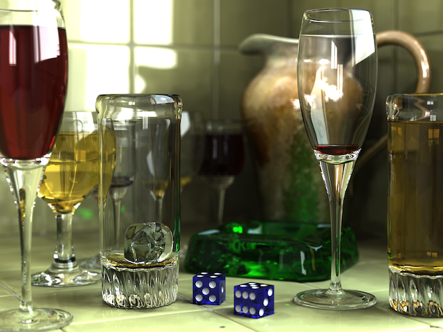
Source: Gilles Tran - http://www.oyonale.com (Public Domain)

This blog post will just offer a really basic introduction on the topic of how such images are created by simulating how light interacts with objects before entering a virtual camera. We’ll be more specifically talking about Path Tracing which is a Ray Tracing algorithm based on casting rays from the camera into a scene, and when a ray hits a surface, the ray is reflected in a new direction based on the properties of said surface’s material. This process is then repeated until the ray intersects a light source, at which point the sequence of rays from the camera to the light have formed a “path”. The “bounce” points on the path can then be weighted together to produce the color of the surface first intersected. Keep on reading for more details!

1.1 Resources

Some excellent resources and inspiration on Ray/Path Tracing:

• https://www.scratchapixel.com/ is by far the most accessible resource when it comes to understanding the mathematics behind computer graphics, Monte Carlo methods and Path Tracing. Fantastic site, warmly recommended!
• The light collection algorithm is based on https://github.com/straaljager/OpenCL-path-tracing-tutorial-2-Part-2-Path-tracing-spheres.
• The ray tracer challenge got me started on Ray tracing a few years ago. Based on TDD and code, it really helped me get my head around the basics of ray tracing.
• PBR book is a quite heavy on the math side of things, but also a good resource for more advanced topics.

2. A layman’s introduction to Path Tracing

Before we get started, I should mention that when I set out to write these blog posts, my main focus was using Golang with OpenCL, where Path Tracing just was the really fun and exciting application of the mentioned technology. This first part will nevertheless purely focus on Path Tracing as a concept, in order to set the stage for the more code-heavy parts to follow.

2.1 Basics

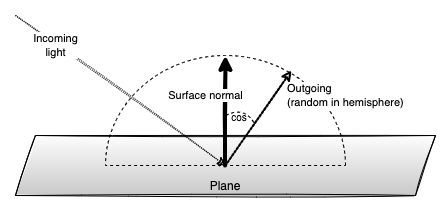
Just a bit of groundwork - how is a ray- or path traced image consisting of ordinary RGB pixels created? How does “rays” cast into a scene relate to pixels in an image? Simply put - one puts an imaginary “image plane” in front of the “camera”, and then one (or in practice - many) rays are cast through each pixel in the imaginary image into the “scene”. The image below from Wikipedia explains it pretty well, just ignore the stuff about shadow ray etc:

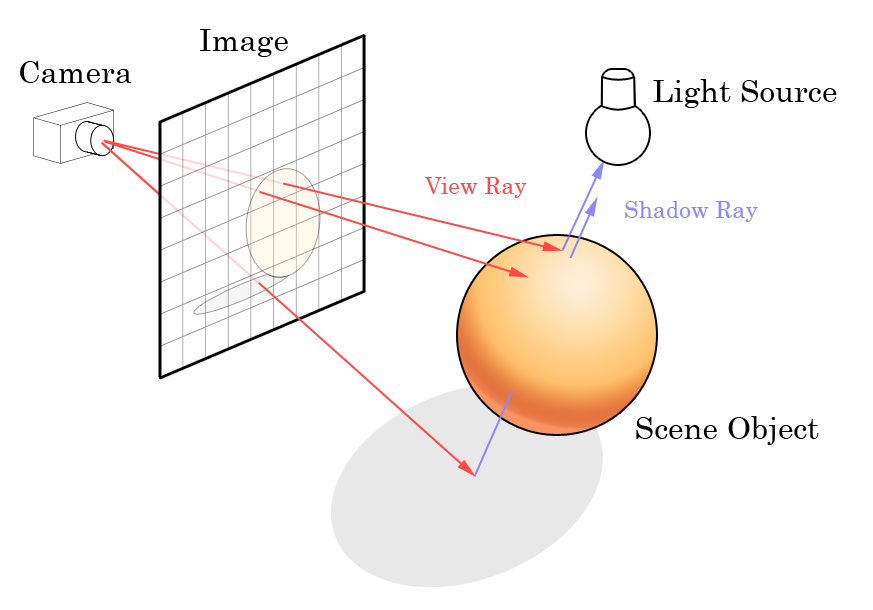
Source: Wikipedia (creative commons)

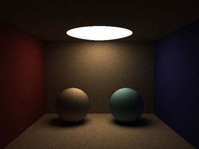
Basically, for each ray cast through a pixel, we’ll check what object(s) that ray intersects, what color the intersected object has, and then return that color. A very basic ray traced image without any other shading can look like this:

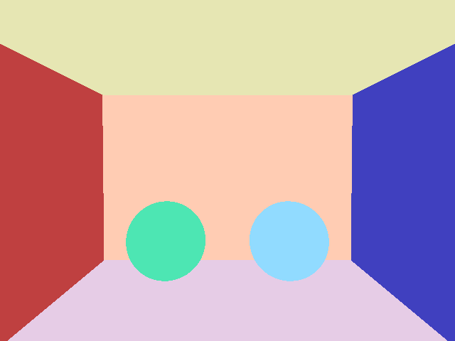
What we see is a box with two spheres in it, where we have simply returned the color assigned to the closest object that the ray cast into each pixel has intersected. This is perhaps ray tracing in its most basic form, from where everything else about these techniques follow.

2.2 Path Tracing basics

Let’s get back to Path Tracing which was briefly introduced a bit earlier. Let’s consider the human eye or the lens of a camera. In real life, we have light sources such as the sun, light bulbs, starlight, moonlight or a candle that continuously emit photons, i.e. “light”. These photons travel through whatever medium that separates the light source from the “camera” such as vacuum, air, glass or water, and eventually will hit something unless the photon travels into outer space.

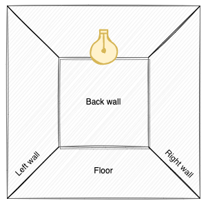
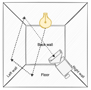
For the sake of simplicity, let’s narrow our scene down to a closed room with a light source in the roof:

If we add a camera to the scene, the “image” seen by the camera is made from light directly or indirectly entering the camera lens, where the color is determined from the wavelength of the light.

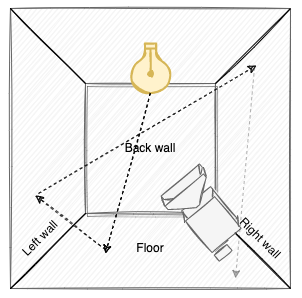
From a purely physical/optical perspective, this probably makes a lot of sense. However, from a computational perspective, simulating light this way in a computer in order to create an accurate image is ridiculously ineffective. We’d probably need to track millions or even billions of light rays originating from the light in order for enough ones to enter the camera lens for an accurate image to be created. After all - the camera lens is extremely small compared to the overall volume of the room:

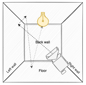
Therefore, the basic Path Tracer implementation flips the coin and instead lets all “rays” originate from the camera, bounce around the scene, and hopefully a requisite fraction will intersect a light source. The “path” in Path Tracing stems from how the primary ray shot into the scene bounces around the scene as secondary rays, which together forms a path of rays where each intersected surface or light source will contribute color to the pixel.

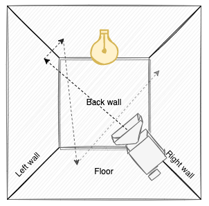
This approach also suffers from most rays not intersecting a light, effectively contributing darkness to the final pixel color. However, since light sources are typically much larger than camera lenses, while still ineffective, casting rays from the camera is vastly more efficient than casting rays from the light source.

As probably evident, we’ll need to perform the operations above many times per pixel in order to get an accurate result, which I’ll get back to shortly in the little section on Monte Carlo methods.

2.3 The Cornell Box

What’s that box-like image anyway? In many path- and ray tracing applications, a so-called Cornell Box is used to determine the accuracy of rendering software. It’s also neat because since its closed, all rays cast will always bounce up to their max number of allowed bounces (such as 5) or until a light source is hit.

2.4 Advantages of Path Tracing

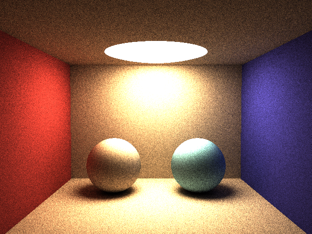
Let’s take a look at a high-res render of our cornell box with three spheres, where the closest one is made of pure glass:

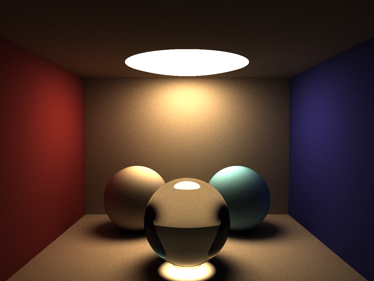
This simple rendered image showcases a few of the advantages Path Tracing has over traditional Ray tracing when it comes to indirect lighting and natural light travel:

• Look at the color of the spheres on their sides facing the left and right walls respectively. Note how the left sphere has a reddish tint caused by light being reflected from the red wall onto the sphere. The same applies on the other sphere, where that blue/purple wall clearly is reflecting light onto the turquoise right sphere.
• Soft shadows. In a simple ray-tracer, creating nice-looking soft shadows is a computationally expensive operation where one needs to cast a large number of extra rays between the surface and random points on an area light source and for each one check if something obstructs the path between the intersection and the point on the light source. In our Path Tracer, we basically get perfect soft shadows for free given the stochastic nature of how light bounces on our diffuse surfaces where some may - or may not - hit a light source. A shadow in the Path-traced image above is simply an effect of having pretty few of the total number of samples for a pixel bounce into the light.
• Caustics. This is the phenomena of light being concentrated by transparent or reflective materials onto surfaces. For rays cast into the spot below that glass sphere, most of the ones bouncing upwards will end up in the light source given how light refracts in a sphere of glass, which means many samples will hit the light source and also contribute a lot of light for the final color of that pixel.

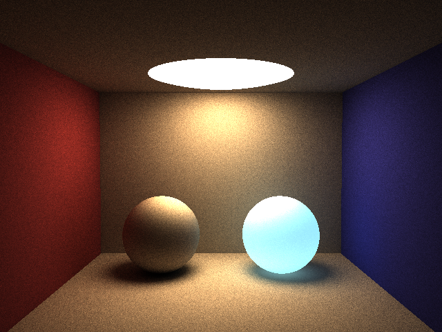
We get all the above due to the Path Tracing algorithm simulating light and color “transport” in a (sufficiently) physically accurate way. In particular, how different materials reflect, absorb and/or transmit light is a huge topic which lot of very smart people have spent time defining algorithms and mathematical models for. In our little path-tracer, we’re mainly dealing with perfectly diffuse materials that will bounce any incoming ray into a new direction in the hemisphere of the normal of the intersected surface. Here’s a very simple example of how a different surface “bounce” algorithm that reflects light a more “narrow” cone produces a result where surfaces get a metallic-like semi-reflective surface:

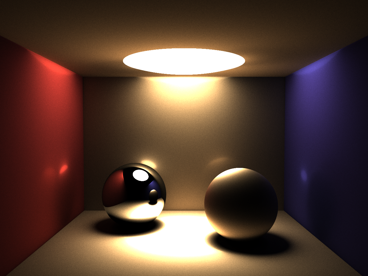
Examine the walls and the right sphere more closely. You’ll probably notice how the more “narrow” cone in which bounce rays are projected, produces a distinctly different result. The image also showcases a reflective sphere, just for fun and giggles.

To summarize, Path Tracing algorithms deals with light transport in a way that gives us much more natural looking images than basic ray tracing, but at the expense of being computationally expensive. More on that soon!

2.5 Computing the final color of a pixel

There’s a group of fancy methods known as Monte Carlo methods which are based on the principle of obtaining an approximate result given repeated random sampling. In practice, these Monte Carlo methods are often much easier to implement than describe from a mathematical point of view.

A commonly used example is determining the average length of a person in a population, let’s say the population of Sweden. You can send your team out with measuring tapes and measure all ~10.4 million Swedes, add all those centimeters together, and finally divide the sum by 10.4 million to get the result. Let’s say 170.43 cm. However, doing this would be extremely time-consuming. Instead, we could use a Monte Carlo method and pick for example 2000 random Swedes to measure, add their lengths together and divide by 2000 - we’re very likely to get a result pretty close to 170.43 centimeters. This is similar to how gallups work and polls work. The key factor is to sample a truly unbiased random selection.

In our particular use case, the same principle applies to tracing photons. We don’t need to trace every single photon entering the camera lens, we can make do with a limited number of samples, as long as they have travelled from the light source, interacted with the scene, and (some) have entered camera in a sufficiently truly random way. In practice, we need to sample each pixel of our image a large number of times, since each bounce on the intersected (diffuse) material will be projected in a random direction in the hemisphere of the object’s surface normal and - given enough samples - will hit other surfaces and light sources in a statistically evenly distributed way. Remember, a pixel is a single pixel in the final image with an RGB value representing its color. A sample also produces an RGB color, but only for a single ray cast through that pixel and bounced around, collecting some light (or not). And we’ll need many random samples for each pixel to obtain an accurate color. If we use too few samples, our approximation will be off which produces noise in the final image, a problem we’ll take a look at in the next section.

Does this sound awfully complicated? It’s not. To obtain the final color for a pixel, we collect a large number of samples, add them together, and finally divide their sum by the number of samples.

finalColor = sum(samples) / length(samples)

2.6 Noise!

How many samples do we need? Having too few samples is the cause of the “noise” commonly associated with Path Tracing performed with too few samples per pixel to produce a sufficiently accurate result. Here’s a sequence of images produced with an increasing number of samples per pixel:

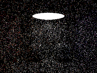
1,2,4,8,16,32,64,128,256,512,1024,2048 samples

In order to get an image without any significant noise (variance approaches 0), we clearly need many thousand samples per pixel, which is one of the main reasons Path Tracing is computationally expensive. For a FullHD 1920x1080 image with 5000 samples per pixel, we’ll need to do over 10 billion samples. And since we bounce the ray of each sample maybe 5 times, where each bounce requires a ray / object intersection test per scene object, even a simple scene such as our Cornell Box will require tens or even hundreds of billions of various computations. This is one of the reasons Path Tracing - while conceptually originating from the 80’s - wasn’t practically useful until CPUs (and nowadays GPUs) got fast enough many years later.

2.7 Computing a color sample

Let’s take a closer look how the color of a single sample for a ray that (eventually) hits a light source is computed using some actual numbers.

In order to determine the color of one sample for a given pixel, we need to calculate how much color each bounce contributes to the final sample color. The data and algorithm for this is remarkably simple: We’ll need the intersected object’s color and the cosine of the OUTGOING (random in hemisphere) ray in relation to the intersected object’s surface normal.

Each bounce’s “contribution” is accumulated into a 3-element vector for Red Green and Blue (RGB) called the mask. The mask is always initiated as pure white 1.0 1.0 1.0 and each bounce will then update the mask using this formula:

psuedo code:

for each bounce, until a light is intersected or MAX n/o bounces have occurred
    mask = mask * bounce.color * bounce.cosine

We multiply the color of each bounce with the cosine of the outgoing ray in relation to the surface normal as a kind of importance sampling, since light projected away from a diffuse surface will be greater if close to its surface normal. Mathematically, we do dot(surfaceNormal, outgoingVec) to obtain the cosine, and the smaller the angle, the closer to 1 the cosine value becomes, hence giving the color of that bounce more “weight”. Needless to say, if no light source was intersected until the max number of bounces occurred (I usually allow up to 5 bounces), then those bounces will only contribute [0.0 0.0 0.0] - i.e. a black sample - towards the final pixel color (which, just as a reminder, is based on monte-carlo integrating a large number of samples).

Time for some numbers. We’ll look at actual debug output for a single ray cast through the pixel that strikes the left-hand side of the left sphere, bounces to the left wall, then over to the right wall before finally entering the light source in the ceiling.

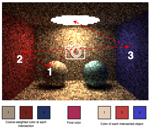
Remember, the formula used is mask = mask * object color * cosine, which means each consecutive bounce will contribute less color, since the mask is always [1.0 1.0 1.0] or less:

What now? The final mask is almost black!?! Here’s when the emission of the light source comes into play. The emission is the strength and color of the emitted light. As clearly seen here, the light source “amplifies” the computed mask in order for the sample color to become reasonably bright. Usually, RGB colors in decimal form are floating-point numbers between 0.0 -> 1.0, but for emission, we’ll use much larger numbers. For this scene, the light emission has RGB [9.0 8.0 6.0]. Why is this even necessary? The reason is again - most diffusely reflected secondary rays will not hit a light source, meaning that the absolute majority of samples will only contribute black color to the final pixel color. Therefore, we need to let the ones that actually intersects a light source a lot of light, otherwise the scene would become way too dark.

So, to get the final sample color, we multiply the mask by the emission: color = mask * emission

[0.666599 0.175565 0.345644] = [0.074067 0.021946 0.057607] * [9.0 8.0 6.0]

There we have it, as seen in the figure above, this particular sample contributed a quite reddish color to the final pixel, even though the base material was a totally different color, since so much color was bled from the red wall.

3. Playing with lights

Note that we can’t graphically represent the exaggerated brightness of the light source - our computer cannot render anything brighter than pure white [1.0 1.0 1.0]. However, if we halve respectively double the emission, the resulting images are noticeably different:

The light in the roof stays pure white though. Note that light sources in this Path Tracer are given no special treatment. They’re intersectable objects just like any other scene object, with the sole difference being that they have a non [0.0 0.0 0.0] value for emission. If we give the right sphere a small amount of emission, it turns into a really dim light source:

We can experiment a little more with light sources. First, an example where we’ve added a small but bright light source between the spheres:

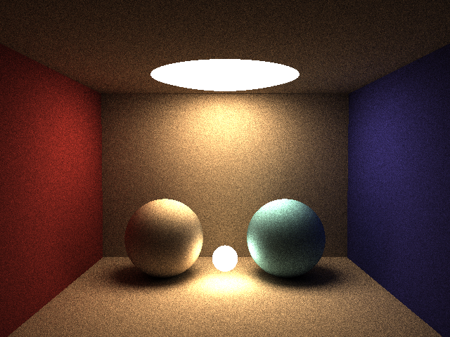
Note the new highlights on the sphere’s inner sides, but also that the new light source doesn’t result in any clearly visible shadows since the roof light already provides good illumination on the walls where shadows otherwise would have been projected.

By removing the roof light source, the result is very different:

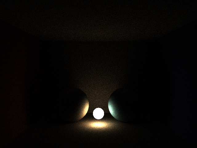
The light is small and partially obstructed, causing most of the walls to stay almost pitch-black since so few of our rays cast from the camera against the walls ends up hitting that tiny light source.

Spotlights are cool, and we can combine a small spherical sphere as a really strong [72.0 64.0 48.0] light source with an open-ended cylinder around it:

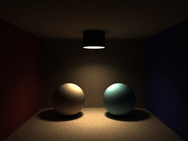
The lighting looks pretty nice with slightly harder shadows and some distinct highlights directly beneath the spotlight, while walls and roof are much more dimly lit since much fewer rays have bounced into the partially obstructed light sphere. This image also showcases another problem with small and partly obstructed light sources with Path Tracing. The image above is quite noisy, even though it uses a whopping 8192 samples! Again - a really bright, but small and inaccessible light source, results in the absolute majority of samples to only contribute black, while the few ones that does intersect the light is really bright, causing inconsistent results which means noise in the image.

There are advanced techniques to partially mitigate noise and reduce the number of required samples such as importance sampling where the previously uniform random sampling is modified to sample more rays “where it is more important”, which means fewer samples will be needed. Another really cool technique is bidirectional path tracing where each sample consists of two (random) paths - one from the camera and one from the light source that’s connected to form a long path from light to camera, which means many more samples will contribute. However, both techniques - while reasonably simple on a high level - are actually very complex and are definitely out of scope for this blog post.

There’s loads of fun one can do with shapes and lights, especially with a path-tracer that supports more types of primitive objects such as cylinders (spotlights), cones (lamp screens), and boxes - and of course plain triangle groups that can be used to represent arbitrary 3D models. Remember, a professional path tracer supports many additional types of light sources, primitives, cameras and features such as depth of field, reflection, refraction, physically correct materials, fog etc.

4. Final words

That about sums it up for the first part of this little blog series. A very quick & dirty layman’s introduction to Path Tracing. I warmly recommend taking a look at the resources listed at the top, written by people who really knows their stuff and which goes into great detail about how these things really work. Nevertheless, I hope this little introduction gave a bit of insight into the topic.

The next installment takes a closer look at using OpenCL with Go!

Until next time,

// Erik Lupander